1.Overview
RTA is a multi-channel Real Time Analyzer for audio signals. It provides time and frequency domain analysis tools to measure RMS or peak levels, frequencies, THD, delays, magnitude, and phase responses. A built-in signal generator provides sine tones, sweeps, and pulses and various noise signals. Using a file player recorded signals can be analyzed.
2. Real Time Analyzer Components
The Real Time Analyzer (RTA) is a tool used to measure and analyses sound waves in real-time. RTA typically consists of several features, that are grouped into various categories to help you navigate and utilize the tool effectively.
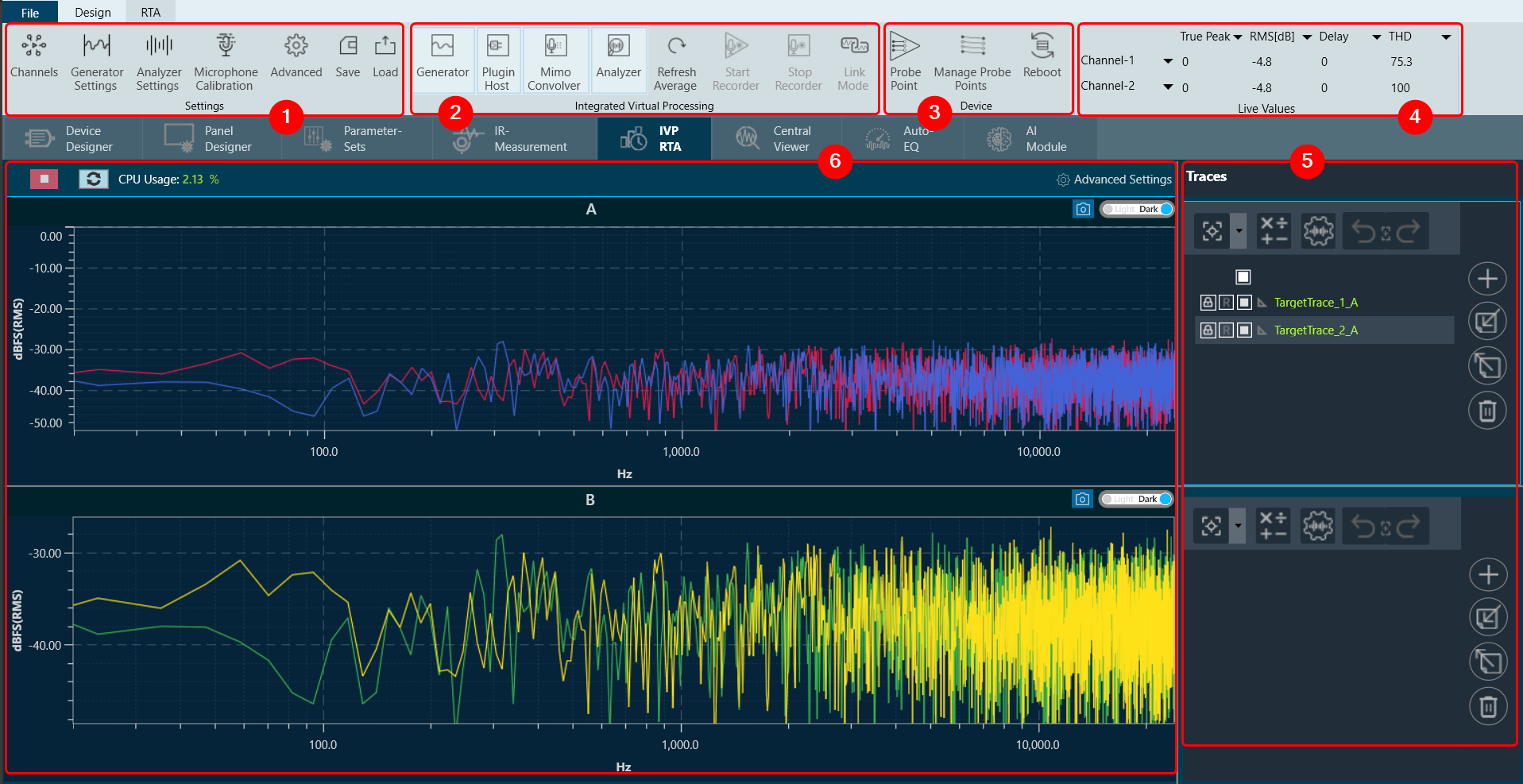
Following are components of Real Time Analyzer:
1. Settings: In an RTA (Real Time Analyzer) window, you can configure various types of settings, that includes:
- Channels Settings
- Generator Settings
- Analyzer Settings
- Microphone Calibration
- Advance Settings
- Save RTA Settings
- Load RTA Settings
For more details refer RTA Settings.
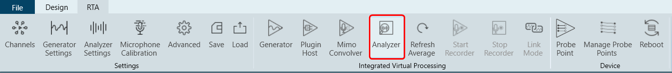
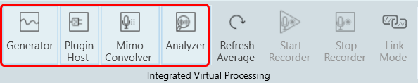
2. Integrated Virtual Processing: In the Integrated Virtual Processing group of an RTA (Real Time Analyzer), you can find various types of processing options that allow you to generate and analyze the audio data. For more details refer Integrated Virtual Process.
Below are the processing options included in RTA.
- Generator
- Plugin Host
- Mimo Convolver
- Analyzer
- Refresh Average
- Start Recorder
- Stop Recorder
- Link Mode
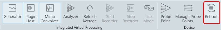
3. Device: This group enables you to manage the probe points of your device. Additionally, it supports the streaming of data from any point in the signal flow back to GTT, allowing for analysis, recording, or reuse of the data within IVP. Below are features included in the group.
4. Live Values: In the section, you can easily view the real time values of RMS, THD, Peak, Peak-Frequency, and THD+N for selected two channels. For more details refer to Real Time Data view.
5. Traces: The trace in RTA is a captured measurement curve. Traces provide the ability to plot multiple measurement curves captured at different times on the same graph, allowing for easy comparison of measurements. For more details refer to Traces.
6. Graph Analyzer: This section shows a graph of the audio signal, which enables the analysis of the spectrum of the audio signal. For more details refer to Graph Settings and Measurement.
3.Settings
Below are the settings available for configuration in the Real-Time Analyzer.

When the RTA or Measurement Module is opened, the main window title bar is updated with status information including sound card and analyzer settings information such as
- Selected HOST API
- Selected device
- Sample rate
- Block length
- FFT length
- Analyzer mode
- FFT window
- Averaging
- Banding

3.1.Channels Settings
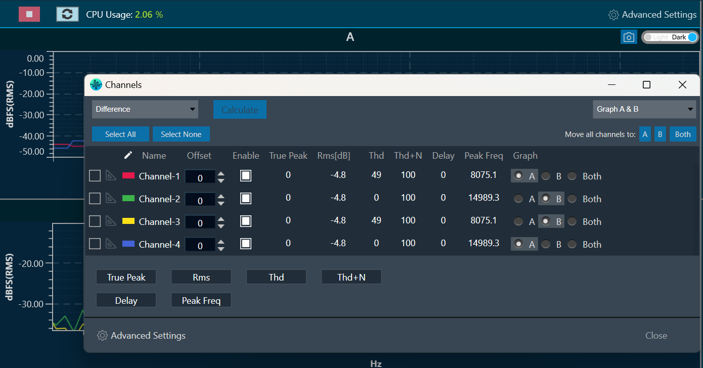
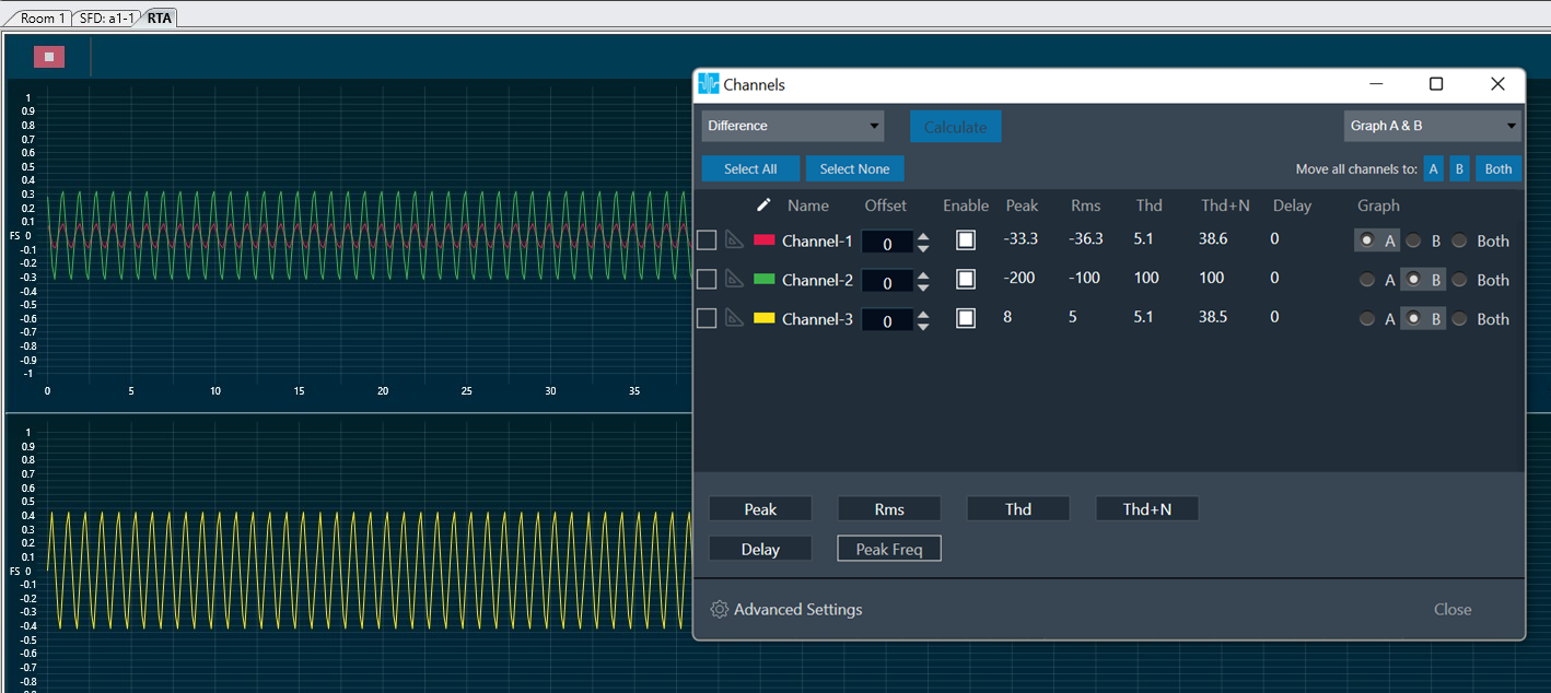
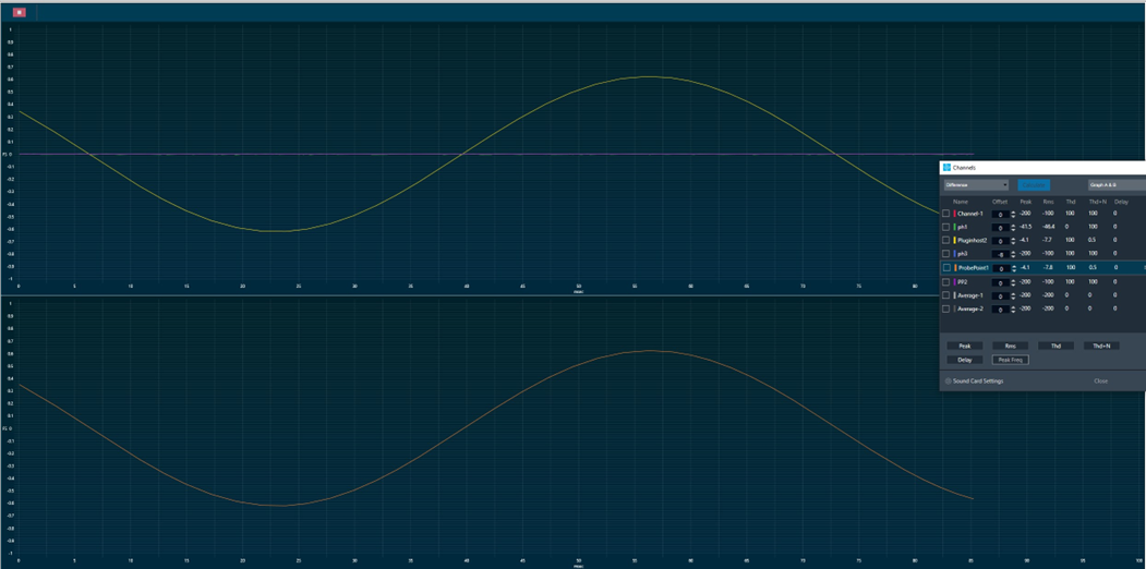
In Channels setting window the numerical measurements are displayed for each channel.
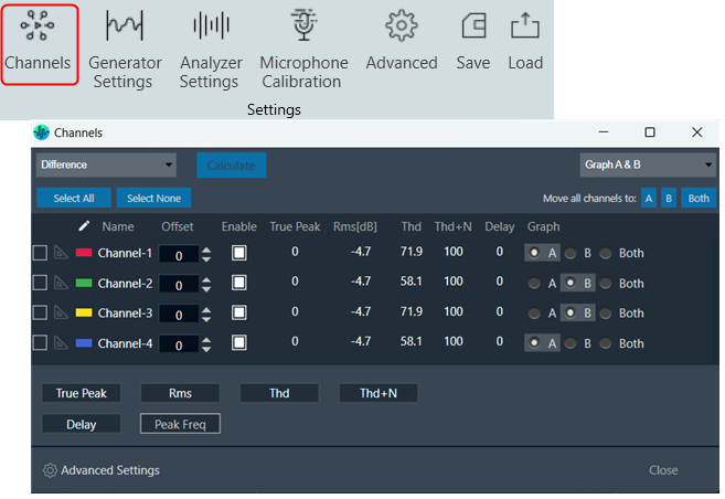
The channel viewer list contains the following columns.
- The first column indicates the colour of the channel. This allows you to change the colour of the channel by clicking on the colour box.
- Name: Display the name of the channel. You can change the name in the Analyzer Settings dialog box.
- Offset: +/- Db shifting of measured and math operated channels.
- Enable: Channel enable and disable allow on display graphs on Analyzer window.
- Peak: The peak amplitude of the current block of analyzed audio samples.
- Rms: The sound level meter value, unit as set in the Analyzer Settings (dBFS, dBV, dBSPL) with selected Weighting (A B C D).
- Thd: Total harmonic distortion in percentage (%).
- Thd+N: Total harmonic distortion plus noise in percentage (%).
- Delay: This value is calculated if Analyzer mode is set to ‘Delay’. The delay measurement is done by cross correlation between a reference channel and a channel which contains the reference signal which went through a certain path (example: amp – speaker – microphone).The delay can be calculated using the position of the maximum within the correlation result.
- Peak Freq: The frequency of the maximum level in the measured spectrum in Hz.
- Graph: Radio buttons allow you to quickly select the graph that displays that channel
By using the Peak, Rms, Thd, Thd+N, Delay, and Peak-Frequency buttons, you can select which values to display in the list.
In addition to assigning individual channels to specific graphs, you can also perform bulk assignments. If no channels are selected, you can use the “Move all channels to A, B, or Both” button to move all channels, including calculated channels, to the desired graph.
If one or more channels are selected, the same buttons will only move the selected channels to the desired graph.
You can use the “Select All” and “Select None” buttons to check or uncheck all channels, respectively.
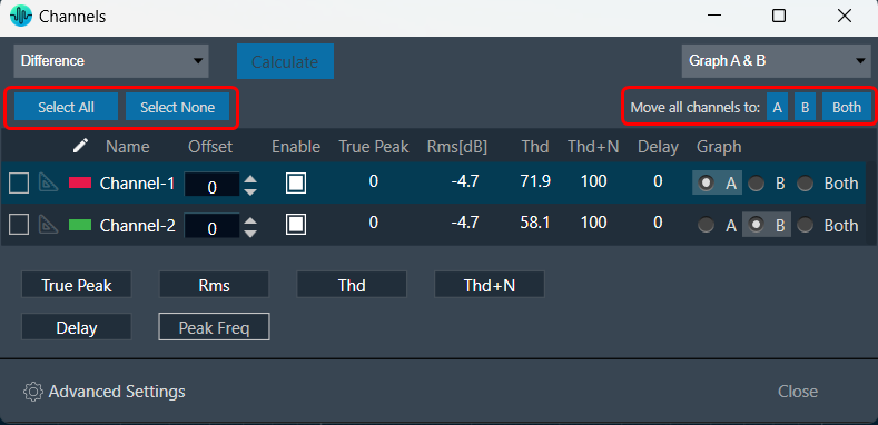
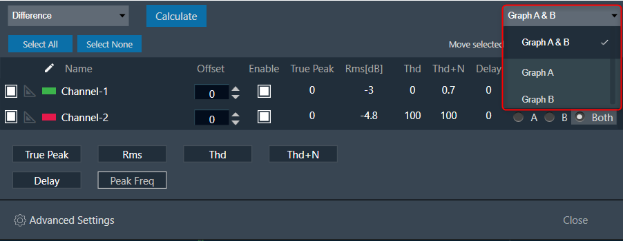
The selector control located at the top left of the window enables you to choose which group of channels to display in the list: all channels (Graph A & B), only Graph A channels, or only Graph B channels.
The channel window is designed to remain on top of other windows and can be resized as needed, making it easy to keep open for value observation while using the RTA.
Click on the “Advanced Settings” to perform additional configuration. For more details about Advanced configuration, refer to the RTA Advanced Settings.
Math operation on Live Channels
To perform math operation:
- Select any two channels.
- Click on the Calculate button to get the math operation result.
Math operated channel is listed on same view.
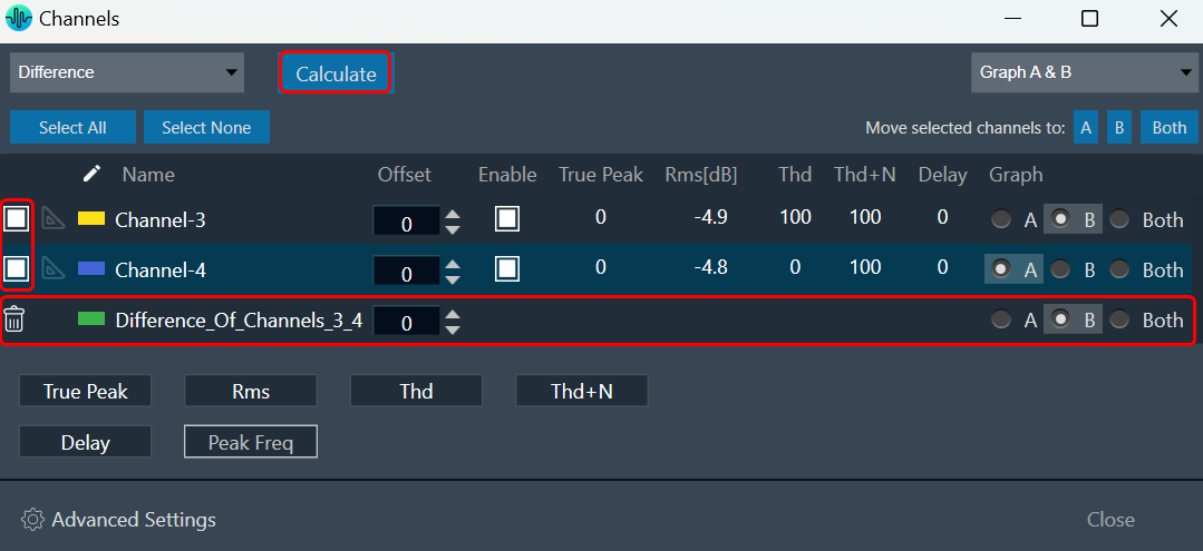
You can delete Math operated channel and as a tool tip you can find which channels are selected for math operations.
Only one Math operated channel can be created for combinations of measured channels.
3.2.Generator Settings
A signal generator is an important feature, which allows to produce specific measurement signals that are then sent to the device or system being tested.
To conduct audio measurements, it is essential to have specific measurement signals which can be produced using a built-in signal generator. You can generate a signal using the “Generator” button in the ribbon bar.
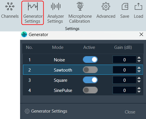
By utilizing the “On/Off” function, you can activate or deactivate a signal. It is possible to generate multiple signals using this feature. The number of signals visible in the “Generator” window is determined by the number of instances specified in the Generator settings.
The gain of the generator signal can be adjusted in 1 dB steps with the Gain control.
To configure the signal, click on the “Generator Settings” to open the advanced RTA setting dialogue box. Here you can configure different generator modes.
On the RTA setting dialogue box, enter the instance value or use the increase and decrease buttons ![]() to change the instance value.
to change the instance value.
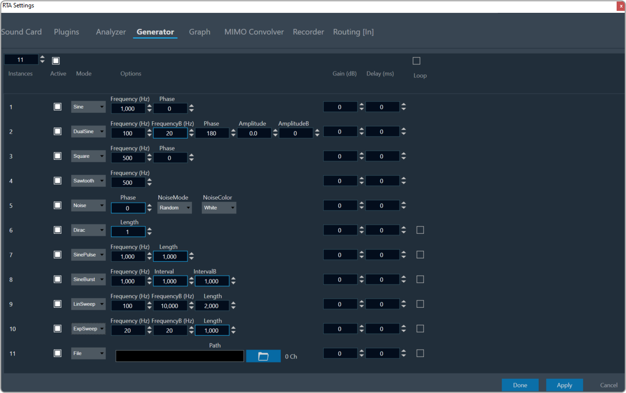
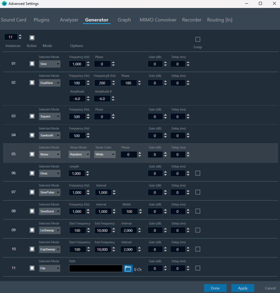
Using “Mode” option, you can select different signals from the drop-down list. The available modes are listed below.
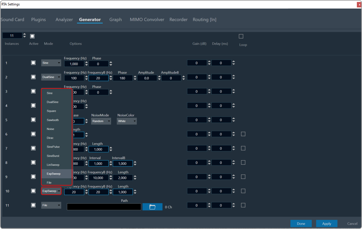
- Sine: A single sine wave adjustable in the audible range between 20 Hz and 20 kHz by SineFreq. The phase between the two output channels can be set by SinePhase.
- DualSine: Two sine waves mixed together to one mono output. The frequencies can be set via DualSineFreq1 and DualSineFreq2, the mixing gains by DualSineGain1 and DualSineGain2.
- Square: Similar to the standard sine wave but shaped as a square wave.
- Noise: This is a stereo noise generator mode. In the Random mode, a regular noise signal is produced. However, when the Noise Mode is set to Pseudo, a multi-sine signal is generated where a sine wave is produced on each frequency bin of the chosen analyzer FFT. The phases of all the sine waves are distributed randomly to create a signal similar to noise.
This mode is used for spectrum analysis of static transfer functions, and it is essential to set the analyzer window function to Rectangle for optimal results, producing very smooth spectrums.
The NoiseColor can be changed between Pink (-3 dB per octave fall off) and White (flat frequency spectrum).
By adjusting the phase the output can be coded in a way so that surround upmixers can pan the signal according to the adjusted angle. The output changes from mono at 0° to L/R uncorrelated at 90° to out of phase at +/- 180°. - Dirac (Dirac Pulse): In this mode one sample wide pulses are generated. The time between two pulses is set by SignalLength.
- SinePulse: This mode generates sine squared pulses. The shape of the pulse is set by SinePulseFreq, the interval between two pulses by SinePulseInterval.
- SineBurst: In this mode sine bursts are generated. The frequency is set by SineBurstFreq, the length of the burst by SineBurstLength and the interval by SineBurstInterval.
- LinSweep: This generates a sine sweep starting from SweepStartFreq and ending at SweepEndFreq. The length of the sweep is set via SweepLength. The frequency progress is linear.
- ExpSweep: Similar to LinSweep only with an exponential frequency progress.
- File: Click on the folder and select the wav file. Based on their selection, the number of channels present in the WAV file will be displayed here. For the selected file, each channel of the selected file will be used as the generator input.
After selecting this mode the user has to adjust the routing settings, hence number of channels depends on the selected file.
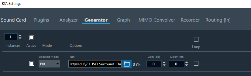
After changing the mode from file mode to any other mode, this routing adjustment has to be adjusted according to the user need and will be signalled by GTT like shown below.

Use “Active” checkbox to either select or deselect all traces. When you select the checkbox at the top, all instance in the window will be automatically selected. Similarly, when the top checkbox is deselected, it will unselect all the traces in the trace window.
Additional Configurations
Loop: If you enable the “Loop” option while using Dirac, SinePulse, SineBurst, LinSweep, ExpSweep, or File mode, the generator will play the chosen signal repeatedly when the Play button is pressed. However, if the loop option is disabled, the generator will play time-limited signals upon pressing the “Play” button.
Delay: You can enter the Delay value. Delay represents the time interval between the input and output of the generator, indicating the time it takes for the generated signal to propagate through the system.
Gain: You can enter the Gain value. The Gain setting allows you to increase or decrease the volume or strength of the generated signal.
The signal generator has a stereo output. This is relevant for signals with adjustable inter channel phase or stereo wav file playback.
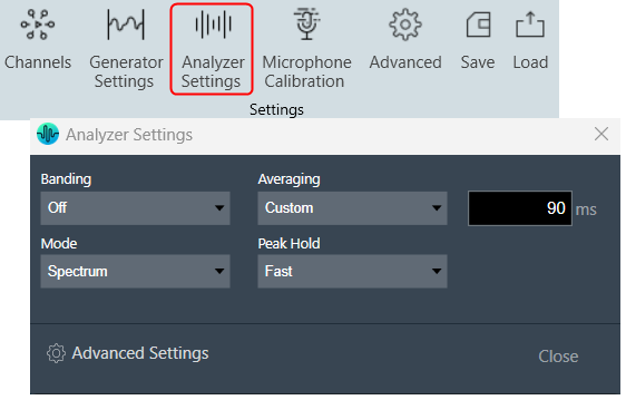
3.3.Analyzer Settings
Using analyzer, you can measure and analyze various aspects of an audio signal. It can be used to measure characteristics such as frequency response, amplitude, distortion, and noise level.
| Settings | Descriptions |
| Banding |
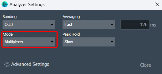
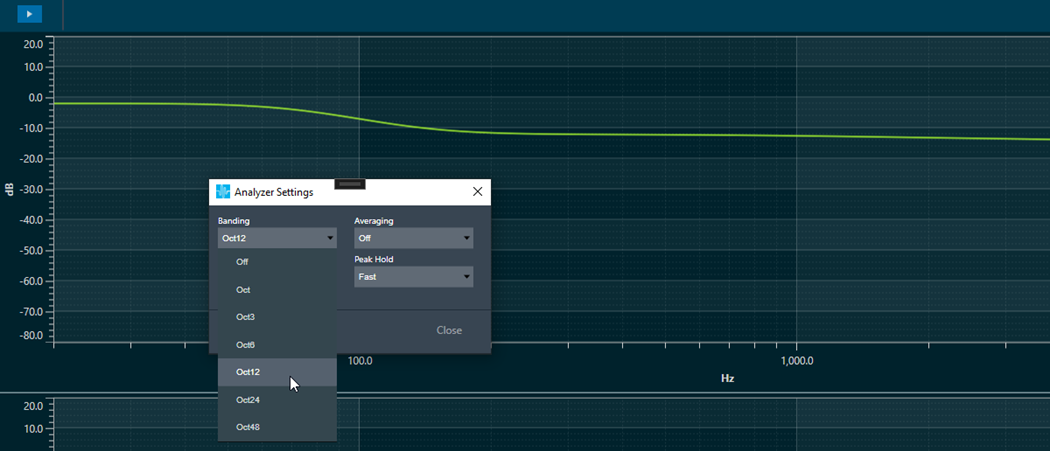
In Spectrum or Multiplexer mode, it is possible to adjust the “Banding”. When the banding is turned off, all frequency bins of the spectrum are displayed, allowing for a highly detailed analysis. However, this setting requires more CPU power as the amount of data that needs to be calculated and displayed increases with the FFT size. Spectrum mode is shown in the example below when Banding is turned off. On the other hand, when banding is turned “On”, frequency bins are grouped together. The width of each group can be adjusted by fractions of an octave, such as Oct12, which means that one band has the width of a 12th of one octave. Spectrum mode is shown in the example below when Banding is turned on. |
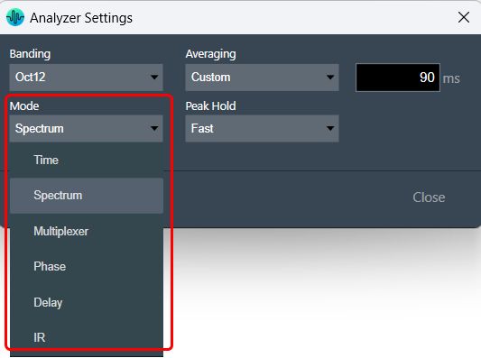
| Mode | Using Mode option, you can select different analyzer mode from the drop-down list. The available modes are listed below.
|
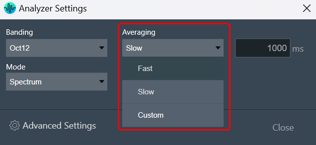
| Averaging |
Depending on the test signal, smoothing of the spectrum over time is required. This can be set by the “Averaging” option.
Following are the averaging options available.
|
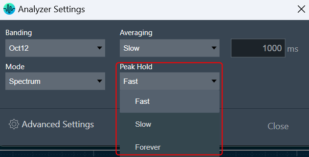
| Peak Hold |
You should be able to select time constant for peak trace. Depending on the time constant setting, the peak hold trace shall show the maximum value which occurred within the defined moving time window.
Peak Hold settings include:
|

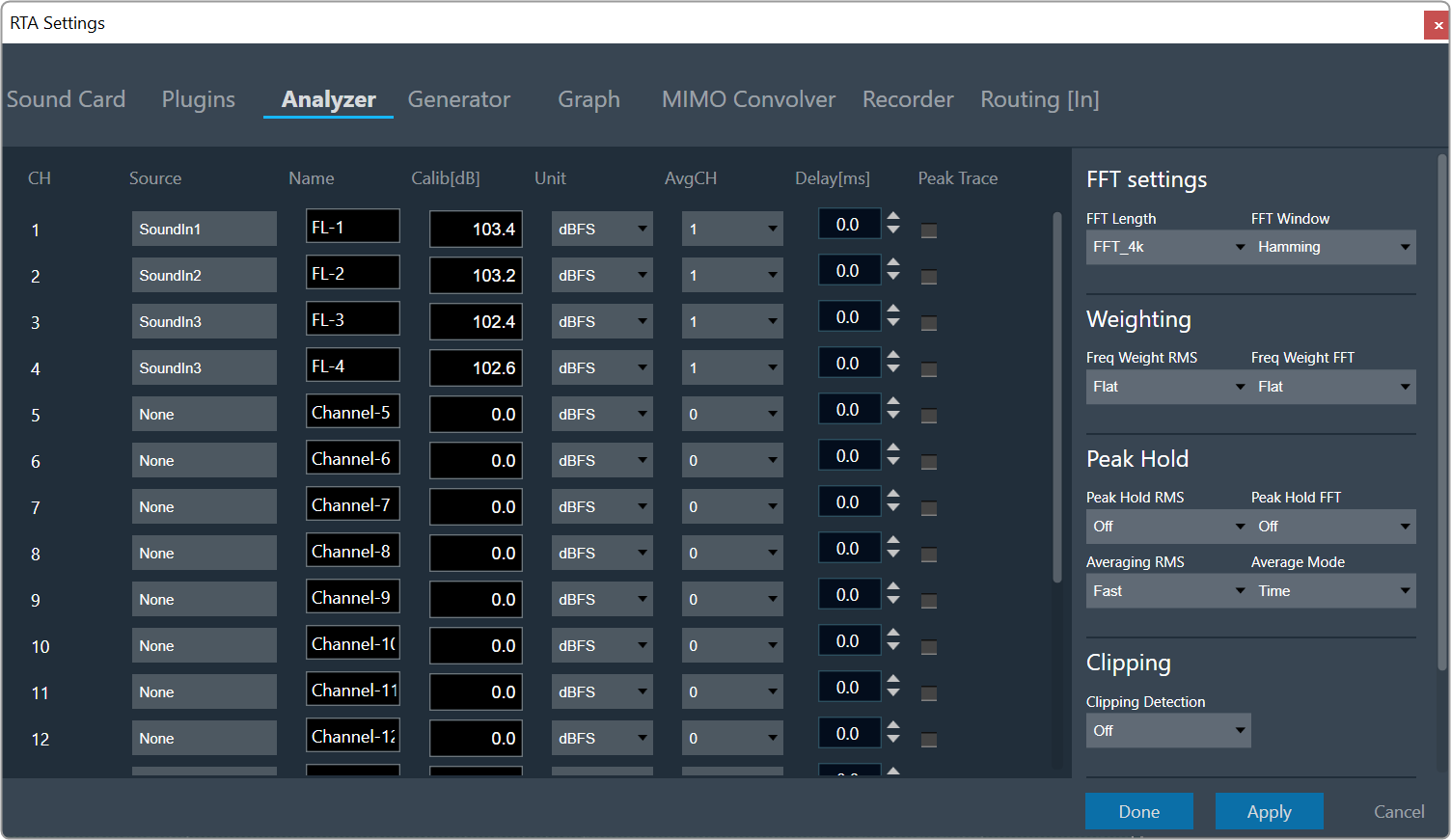
Advanced RTA Setting
Click on the “Analyzer Settings” to open the advanced RTA setting dialogue box. Here you can configure different analyzer settings.
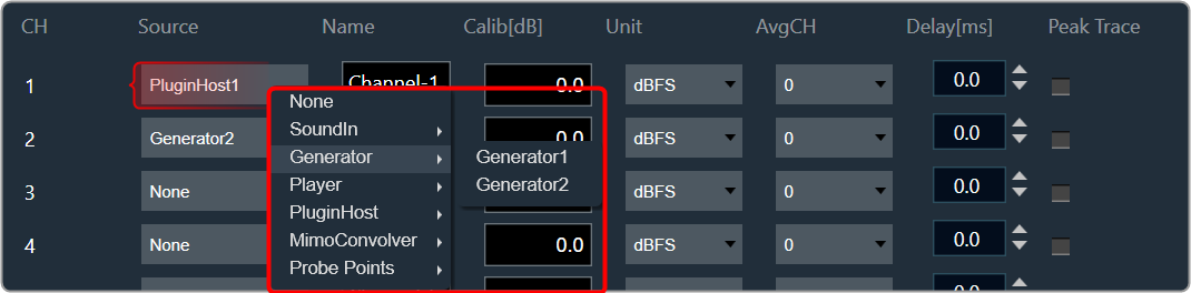
The following modifications can be made in the Analyzer setting window using the channels list:
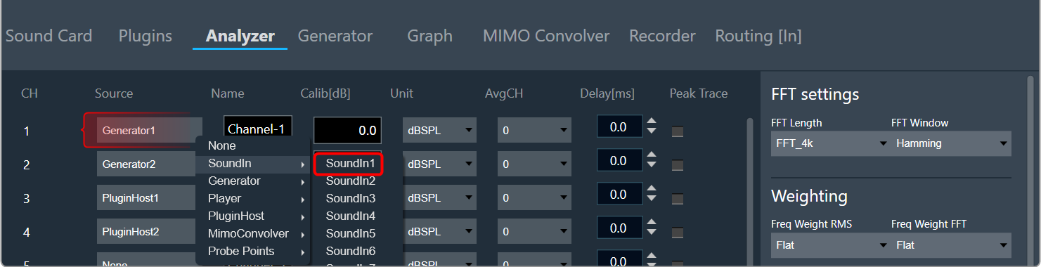
- Source: This defines the input of a certain analyzer channel. By clicking on the control a context menu pops up from which the desired source can be chosen.
If there is no input available, None will be shown as the source by default.

- Name: Enter the name of an analyzer channel. This name appears in the channel viewer and will be set as a default name when storing measurements as traces.
- Calib[db]: When a channel is being calibrated for a certain microphone the determined value appears here. It can also be overwritten by entering a desired value. The unit is “dB”; the analyzer input stream will be scaled by this value.
- Unit: Allows you to set the analyzer source unit. This unit appears later in the channel viewer.
- AvgCH: When the analyzer is in “Multiplexer” mode this control determines to which “Average” channel the analyzer source is added.
When the channel is “0,” it is not included; when it is “1” or “2,” it is added to “Average-1” or “Average-2,” respectively. - Channels 17 and 18 are reserved for the “Average” channels. Here only the name can be edited.
- Delay: Add or subtract time delay in milliseconds. In Phase measurement we can add/subtract time delay to compensate HW and/or acoustic delay.
- Peak Trace: Peak hold trace allows analyzer to display a secondary live trace for each channel showing the highest amplitude values for each frequency. This feature helps to mark the highest amplitude reached at each frequency.
By default all the peak trace will be disabled. This can be enabled using the checkbox available in the analyzer settings tab for each channel.
Click “Delete” in the data context menu of the peak trace in the trace list to reset the peak trace. When a peak trace is deleted, the database will also delete the current peak trace and create a new one.
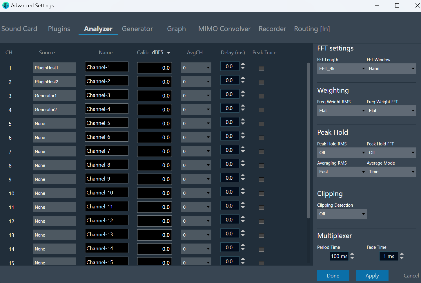
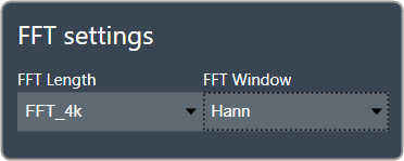
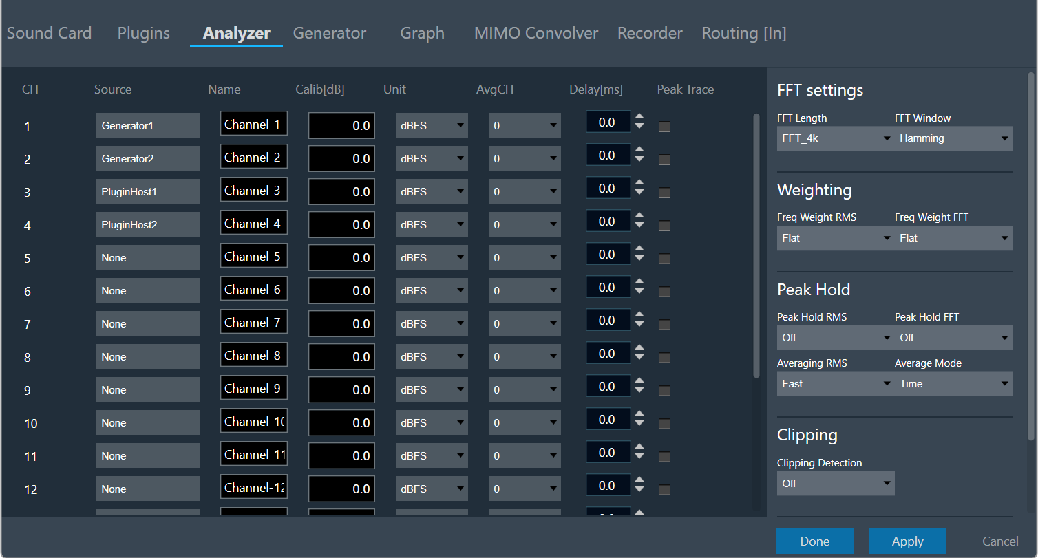
| FFT Settings |
The length of the FFT which is used for the spectrum calculation can be set between starting from 4096 up to 131072 samples (4k to 128k). The higher the value, the finer the frequency resolution of the spectrum. But with increasing lengths the CPU load will increase due to the higher number of calculations and data to plot.
You can specify how a finite data set is extracted from the roughly infinite input data stream using the “FFT Window”. The “FFT Length” determines how the data set is cut out. For more details about windowing, refer to the Window Functions. “Hann” will be the default value for the FFT window. |
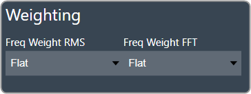
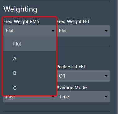
| Weighting |
The Weighting function allows you to select how the input signal is weighted across the frequency range. This can be customized separately for time domain measurements (Freq Weight RMS) and frequency domain measurements (Freq Weight FFT).
For more details about weighting, refer to the A-weighting. |
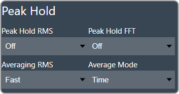
| Peak Hold | The Peak Hold function enables you to independently adjust measurements in the time domain (Peak Hold RMS) and frequency domain (Peak Hold FFT).
Averaging RMS: The time constant for the RMS calculation can be selected under “Sound Level Meter”.
Average Mode: The analyzer mode “Multiplexer”, where multiple channels are added to a single “Average” channel can be set to “Time” and “Freq”.
|
| Clipping |
Clipping occurs when the input signal exceeds the full-scale range of the input sound device. RTA can detect this condition and signal it. There is also an option to exclude the data packet which contains clipped data from the analysis.
Clipping Detection mode includes:
When data are clipped, and the detection is enabled a “DATA CLIPPED” message on the top right corner of the graph is shown. |
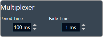
| Multiplexer |
Activating the multiplexer mode to “Time” allows you to set the length of a time slice (referred as “Period Time”) and the time duration for fading one channel into the next (referred as “Fade Time”).
|

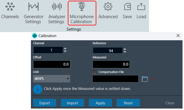
3.4.Microphone Calibration
The purpose of microphone calibration is to convert the soundcard input values, which are typically within the range of +/- 1 (full scale FS), to the actual sound pressure level that is captured by the connected microphone.
To achieve this, a calibration device, such as a pistonphone, is connected to the microphone. This device produces a constant sine tone with a predetermined level, such as 94 or 114 dB.
The level of the microphone signal is measured by the RTA, and the calibration level can be saved for future measurements.
Prerequisites
- In the Analyzer Settings connect the SoundIn channels to the Analyzer inputs.
- Set the “Peak Hold RMS” to “Off”.
- Set the “Freq Weight RMS” to flat (important if the calibration frequency is not 1 kHz).
- Set the “Sound Level Meter” to Slow.
Steps to perform microphone calibration:
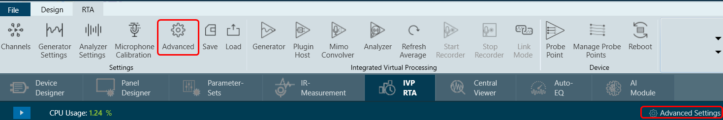
- Navigate to the IVP RTA tab and select Microphone Calibration from the ribbon bar. This opens the Calibration dialogue box.
- In the Calibration box, adjust the channel that needs to be calibrated and click Reset.
- Select the desired unit. Usually the unit of measurement is dBSPL, but for electrical measurements dBV is selected. The selected unit will be applied to all subsequent channels.
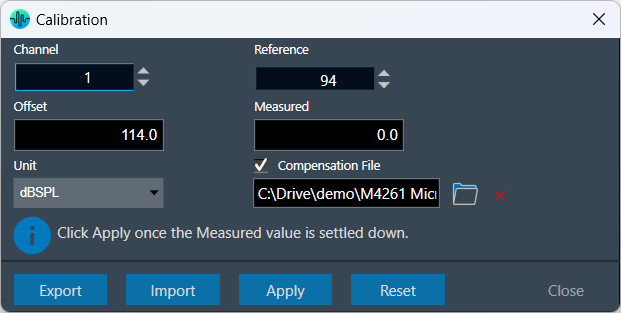
- Attach the calibration device.
- Wait until the “Measured” value has stabilized, and then click on Apply.
- (Optional) Select the Compensation File. This file is provided by the microphone manufacturer and is used to correct the microphone’s frequency response. You can On or Off this correction using the adjacent checkbox. To take the selected compensation file into effect, please restart the analyzer.
You don’t need to click on “Apply” for selecting a compensation file. “Reset” will only reset the offset; it has no impact on calibration file.
The compensation file is only considered for magnitude curve correction; it has no impact on calculated metrics such as sound pressure level (SPL) and total harmonic distortion (THD).
The calibration result is automatically stored in the analyzer settings. They can be modified manually at any time.
Additionally, you can export and import files with calibrated microphones.
- It is possible to import XML/JSON files with calibrated microphones exported from MMIR and IVP/RTA.
- It is possible to export and import JSON files with Channel Number, Offset and mic compensation file of the calibrated microphones.
3.5.RTA Advanced Settings
RTA Settings window is now non modal, you can save the settings and validate without closing It.
RTA Settings dialogue box comprises of the following settings:
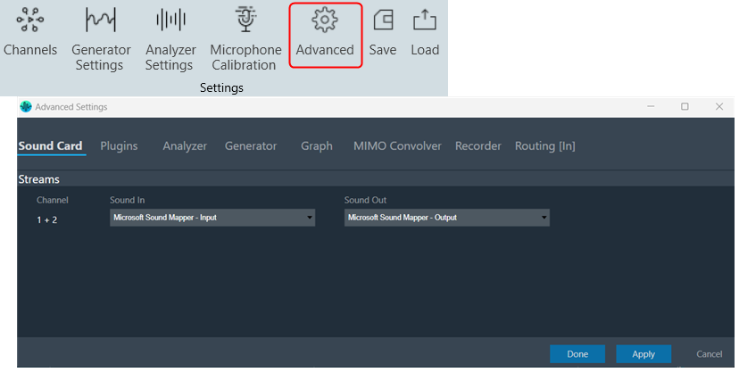
3.5.1.Sound Card Settings
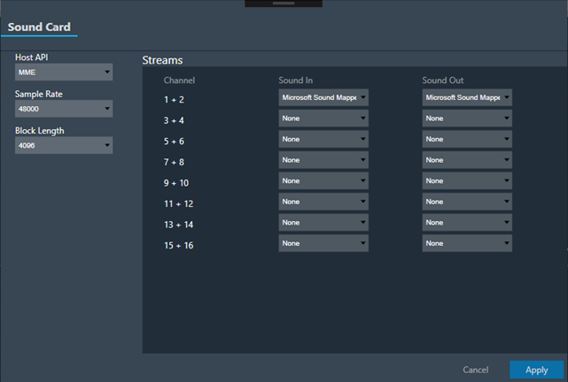
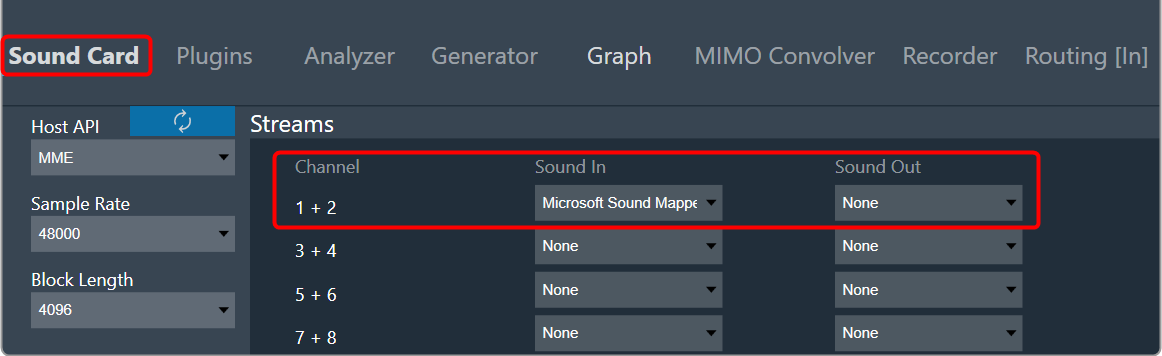
Before you set the “Sound In” and “Sound Out” devices, make sure you have configured sound card settings like Host API (Driver Protocol), Device, Sample Rate and Block length of the sound card. Refer to the Sound Card Configuration to know about configuration details.
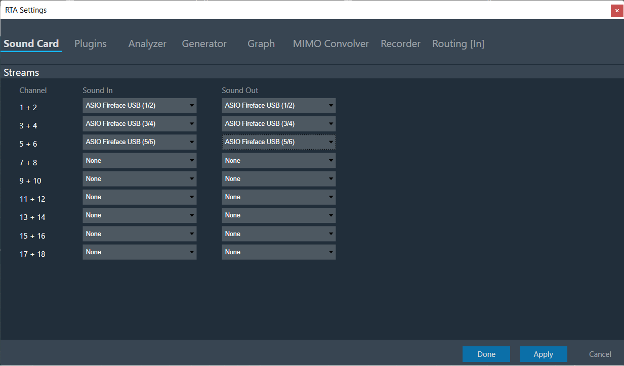
During sound card configuration, RTA channel streams should be automatically assigned with available input and output devices if the user has not already assigned any sound input or output devices to RTA Channel streams.
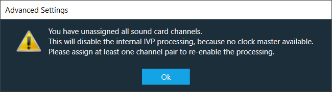
If the user attempts to unassign all sound card channels, a toast message should be displayed with message like “You have unassigned all sound car channels. This will disable the internal IVP processing, because no lock master available. Please assign at least one channel pair to re-enable the processing”.
After selecting a Host API, it is necessary to choose the Sound In and Sound Out devices.
If no device is selected, RTA will operate in a silent mode, which can be useful for verifying generator modes or analyzing pre-recorded measurements from a .wav file.
All devices are available as two-channel devices. The stream area displayed the Channel column, indicating the mapping of Sound In or Sound Out devices to specific channel pairs. These channel pairs, labelled as Sound In 1 to 16 and Sound Out 1 to 16, are accessible in the analyzer and routing settings. You can select these channels from the context menu to establish connections between sound card channels and RTA processing blocks.
In the example above the mapping is configured as follows:
- SoundIn1, SoundIn2: Analog (1 + 2)
- SoundIn3, SoundIn4: Analog (3 + 4)
- SoundIn5, SoundIn6: Analog (5 + 6)
- SoundOut1, SoundOut2: Analog (7 + 8)
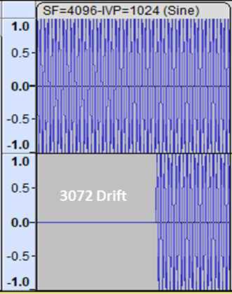
In case the device block length is higher than your sound card block length. It will introduce an additional latency in the signal chain, which will cause a shift in the start position and missing blocks at the end of the recording.
For example, if the device block length is equal to 4096 and sound card block length is equal to 1024, there will be a “drift” of 3-blocklengths or 3072 as you can see below:
If there are any modifications to the Sample Rate, Block Length, or Host API, it is necessary to reconnect the device.
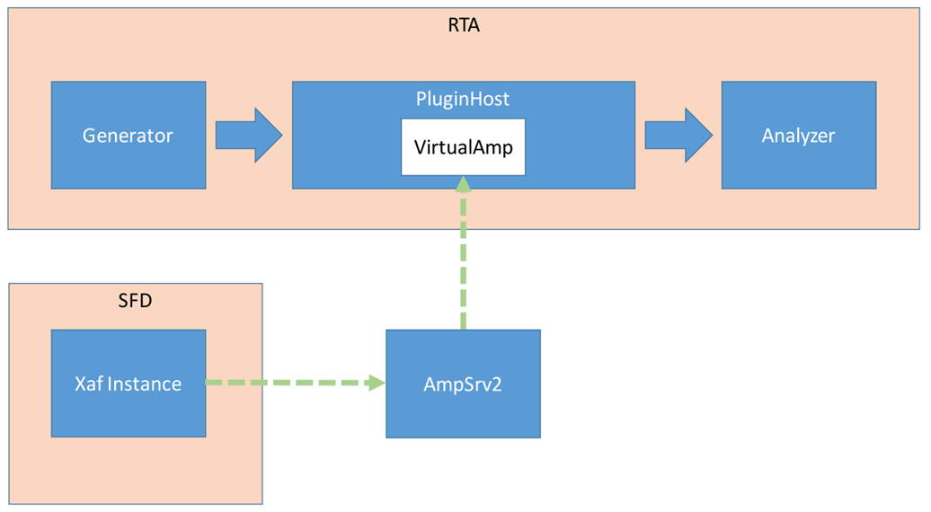
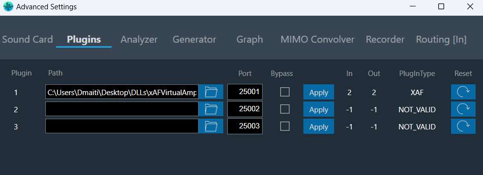
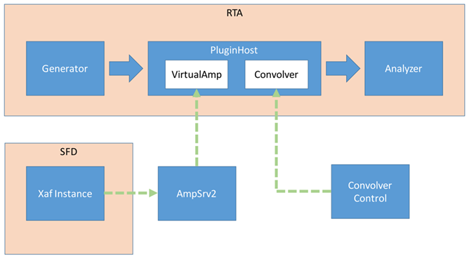
3.5.2.Plugin Host Setting
The Plugin Host is a host for virtual amp dll. The Plugin Host supports up to 3 instances of plugins (virtualAmp.dll in 64 bit), which are executed in series.
The block sizes and sample rate will be determined by the sound card settings and will be applied to all plugins. If the block size of the device/instance does not match the plugin’s block size, the plugin needs to internally handle the block size conversion.
The Virtual Amp does not support sample rate conversion in the current version. If a sample rate conversion is attempted, an error message will be displayed, and the processing will be stopped.
Steps to configure plugin host:
- Navigate to the IVP RTA tab and select Advanced from the ribbon bar. This opens the RTA Settings dialogue box.
- On the RTA Settings dialogue box, select the Plugins tab.
- Click on the folder icon to browse the xAF library path.
- Set port number under the Port box.
- Enable the Bypass option (optional), if you prefer the input to be passed directly to the next plugin or output without undergoing any processing.
- Click on Apply. The number of inputs, number of outputs, and plugin type will be automatically updated based on the provided signal flow. Similarly, you can set remaining plugins.
Click on Reset (optional), to set back all the values in a specific row to their default values.
- Go to the Routing [in] tab.
- Set the inputs for “Plugin Host” (such as Generator1 and Generator2). These inputs will determine the channels from the Plugin Host that will be used.
- Set inputs for “SoundOut” in order to route the PluginHost output channels to the sound card outputs.

- If you want to display the output of PluginHost in RTA (optional), go to the Analyzer tab and select Plugin Host output as the channel source.
- Set the Channel source (such as Generator1, Generator2, PluginHost1, and PluginHost2) to display in chart.
- Once the settings have been updated, click Done.
By default (no flash file available next to the virtualAmp.dll), the number of in-/outputs in the plugin host is -1.
Default Port Number starts from 25001.
Connect to device through Plugin Host
-
Click Plugin Host.
The Plugin host button is disabled until you select a valid plugin host.
- Switch to Signal Flow Designer window, configure signal flow and click on Send Signal Flow. A pop-up message will ask you to reboot device.
- Switch to the IVP RTA tab and click Reboot.
- Switch to Device Designer tab and click on Connect Device to connect to device.

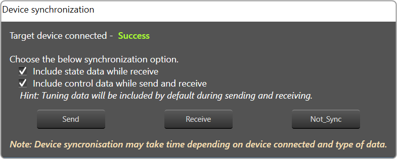
- Device synchronization dialogue box will appear, enable the desired synchronization option, and click Send.
If AmpSrv is unable to connect, close it and retry.
Now you can perform tuning on the IVP RTA.
-
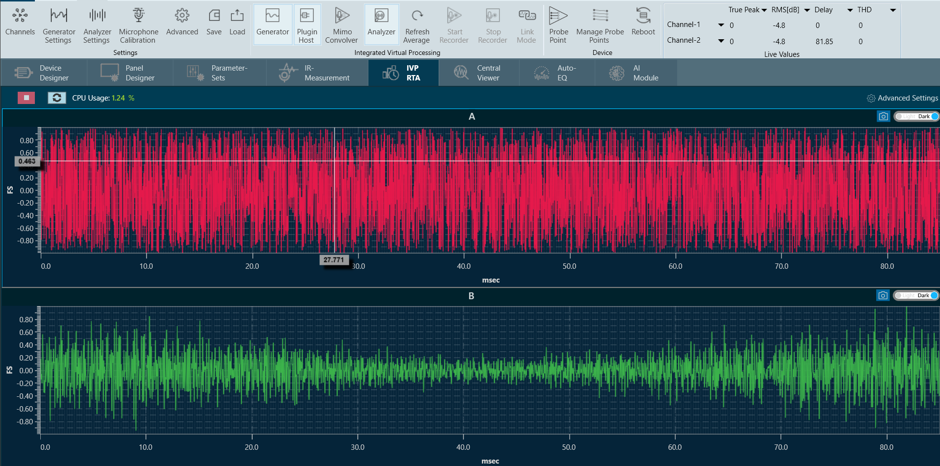
Switch To IVP RTA tab, click on Generator and Analyzer option. On the graph section, the generated signal will be displayed.
- Click on Channels to see the values of each channel. If you want to configure the graph, click on Advance Settings and go to the Graph setting.
3.5.3.Advance Analyzer Settings
Click on the “Analyzer Settings” to open the advanced RTA setting dialogue box. Here you can configure different analyzer settings.
The following modifications can be made in the Analyzer setting window using the channels list:
- Source: This defines the input of a certain analyzer channel. By clicking on the control a context menu pops up from which the desired source can be chosen.
If there is no input available, “None” will be shown as the source by default.
- Name: Enter the name of an analyzer channel. This name appears in the channel viewer and will be set as a default name when storing measurements as traces.
- Calib[db]: When a channel is being calibrated for a certain microphone the determined value appears here. It can also be overwritten by entering a desired value. The unit is “dBFS”; the analyzer input stream will be scaled by this value. Based on microphone calibration unit, this unit will be set. The same unit will be suffixed to Y Axis unit for Spectrum mode graph. Example: dBFS(RMS), dBSPL(RMS) etc.
- AvgCH: When the analyzer is in “Multiplexer” mode this control determines to which “Average” channel the analyzer source is added.When the channel is “0,” it is not included; when it is “1” or “2,” it is added to “Average-1” or “Average-2,” respectively.
Channels 17 and 18 are reserved for the “Average” channels. Here only the name can be edited.
- Delay: Add or subtract time delay in milliseconds. In Phase measurement we can add/subtract time delay to compensate HW and/or acoustic delay.
- Peak Trace: Peak hold trace allows analyzer to display a secondary live trace for each channel showing the highest amplitude values for each frequency. This feature helps to mark the highest amplitude reached at each frequency.
By default all the peak trace will be disabled. This can be enabled using the checkbox available in the analyzer settings tab for each channel.
Click “Delete” in the data context menu of the peak trace in the trace list to reset the peak trace. When a peak trace is deleted, the database will also delete the current peak trace and create a new one.
You should be able to select time constant for peak trace. Depending on the time constant setting, the peak hold trace shall show the maximum value which occurred within the defined moving time window.
Peak Hold settings includes:
- Slow
- Fast
- Forever
3.5.4.Advance Generator Settings
In the advance generator setting window you can configure different generator modes and set the various parameter of the signal. For more details about generator settings, refer to the Generator Settings.
3.5.5.Graph Display Settings
The Graph display setting enables you to customize the appearance and behaviour of a graph or chart. These settings allow you to control the visual aspects of the graph, Min/Max of various parameters, as well as the overall layout style.
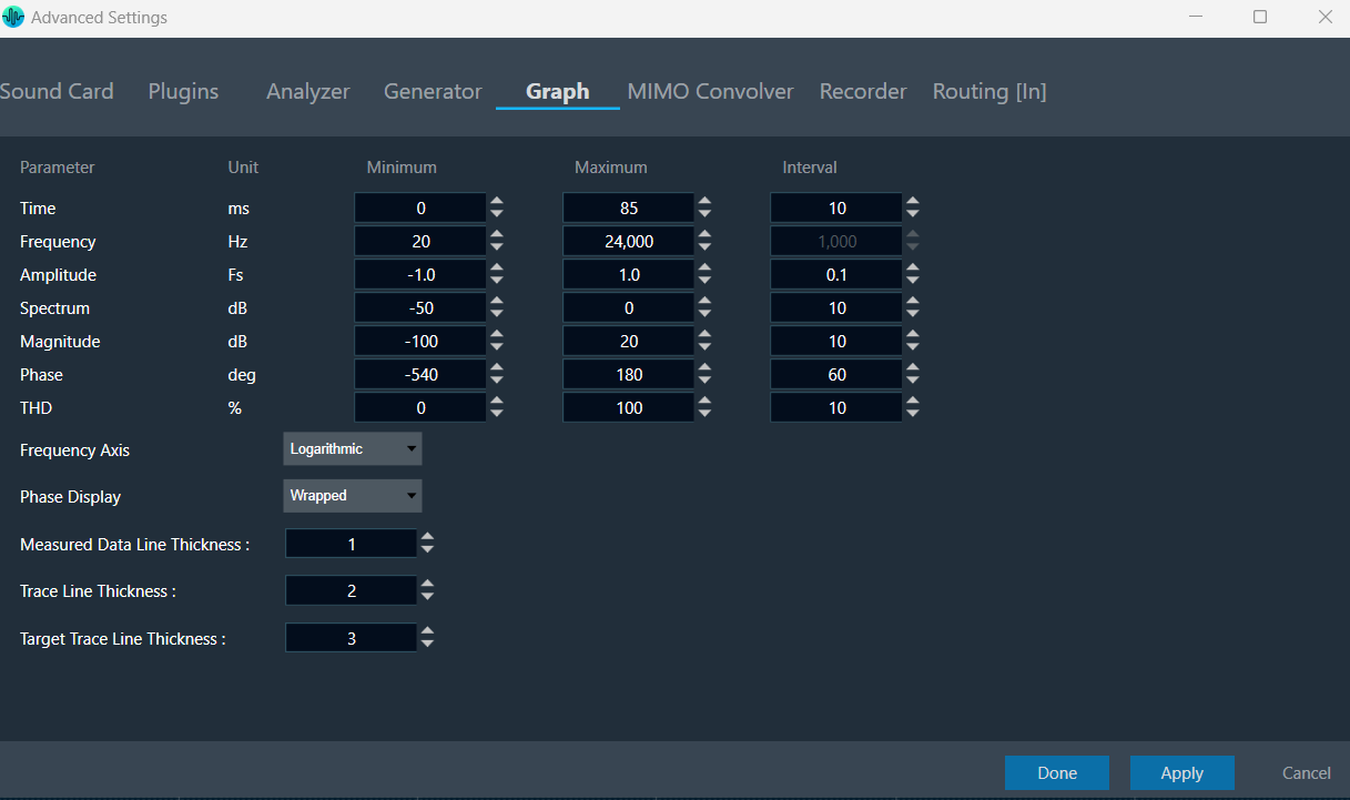
Following are settings you can configure in the “Graph” display.
- Set the Minimum and Maximum value for the Time/ Frequency/ Amplitude/ Spectrum/ Magnitude/ Phase/ THD parameter.
- Interval sets the delta of horizontal/vertical labels.
- Set Frequency axis as Logarithmic or Linear.
- Set Phase display as Wrapped or Unwrapped.
- Set the curve line thickness for Measured Data Line, Traces Line, and Target Traces Line.
After updating the graph settings, click on Done to save the changes. Ensure that values persist when importing or exporting a project.
Interval will be disabled for Log Scale.
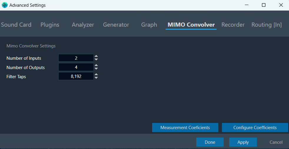
3.5.6.Mimo Convolver Settings
Convolution is the process of multiplying the frequency spectra of our two audio sources: the input signal and the impulse response. By doing this, frequencies that are shared between the two sources will be accentuated, while frequencies that are not shared will be attenuated.
This phenomenon occurs when the input signal adopts the sonic characteristics of the impulse response, resulting in enhanced frequencies that are commonly present in both the impulse response and the input signal.
Steps to configure MIMO Convolver:
- Navigate to the IVP RTA tab and select Advanced from the ribbon bar. This opens the RTA Settings dialogue box.
- On the RTA Settings dialogue box, select the Plugins tab.
- Click on the folder icon to browse the xAF library path.
- Set port number under the Port box.
- Enable the Bypass option (optional), if you prefer the input to be passed directly to the next plugin or output without undergoing any processing.
- Click on Apply. The number of inputs, number of outputs, and plugin type will be automatically updated based on the provided signal flow.
- Switch to MIMO Convolver tab.
- Set number of Inputs, Outputs, and Filter Taps.
You can configure coefficients in 2 ways.
- Configure coefficients in Panel.
- Configure coefficients through virtual prediction.
Configure coefficients in Panel
- On the MIMO Convolver tab, click on Configure Coefficients. The Configure Coefficients panel launches with 2*2 filters.
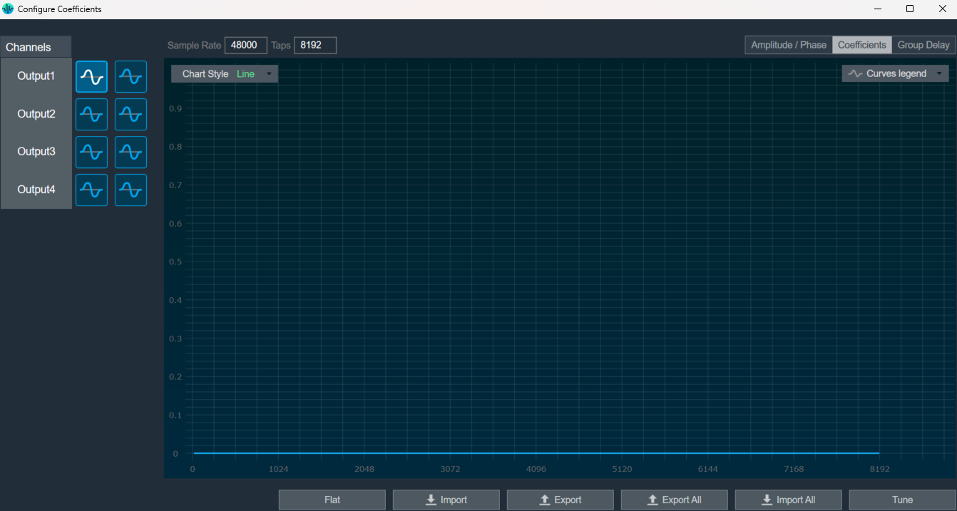
- Adjust the coefficients by either setting them to a flat value or importing them using CSV/XML files.
- Click on Tune, after assigning coefficients.
A toast message “Tuning applied” appear.
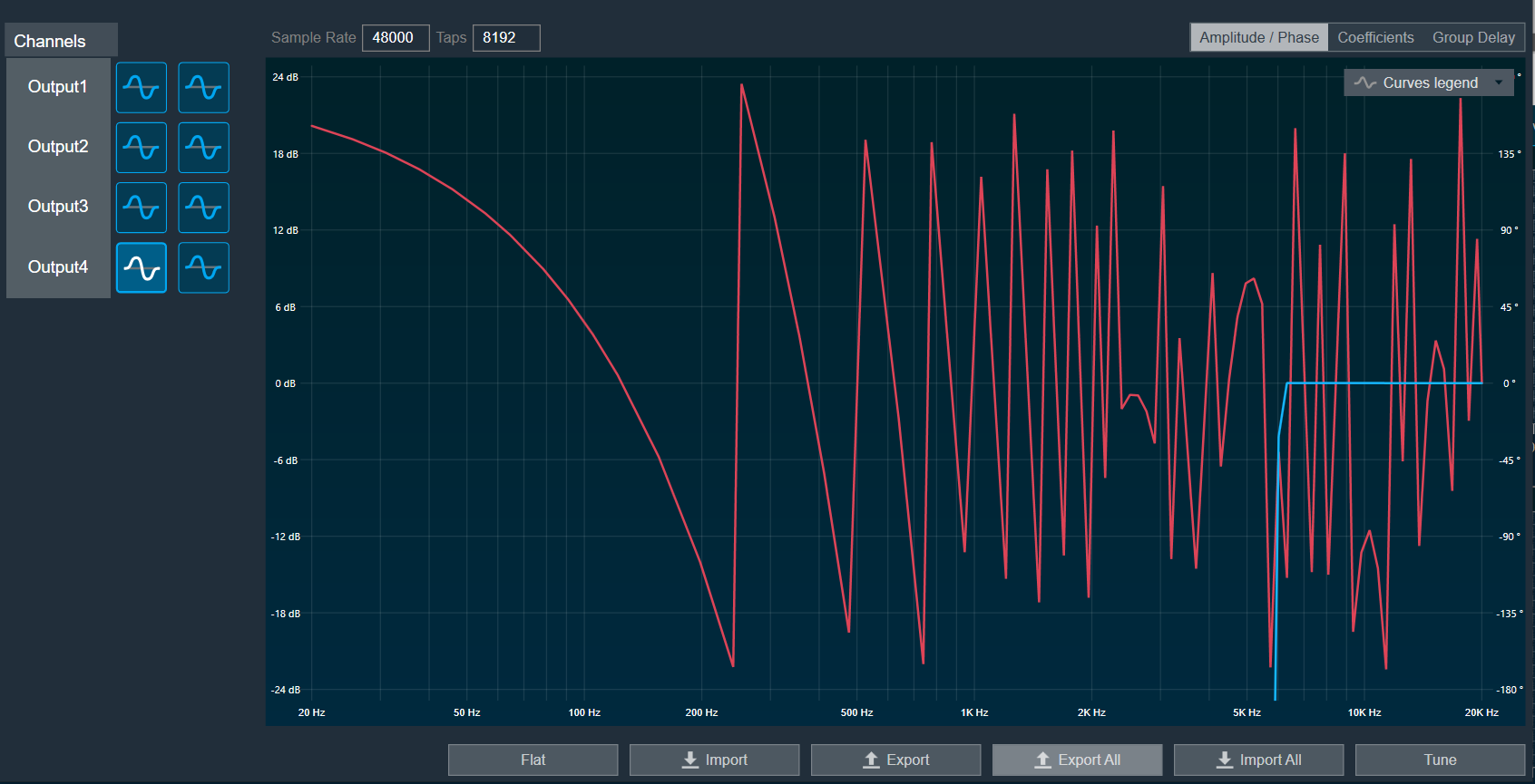
Amplitude/Phase: When the coefficients are given and “Amplitude/Phase” option is selected, the graph display the value.
Coefficients: When the coefficients are given and the “Coefficients” option is selected, the graph displays the values as per below figure. You can change the graph style using the “Chart Style” option.
| Line chart style: when “Chart Style” selected as Line, the Coefficients graph. | 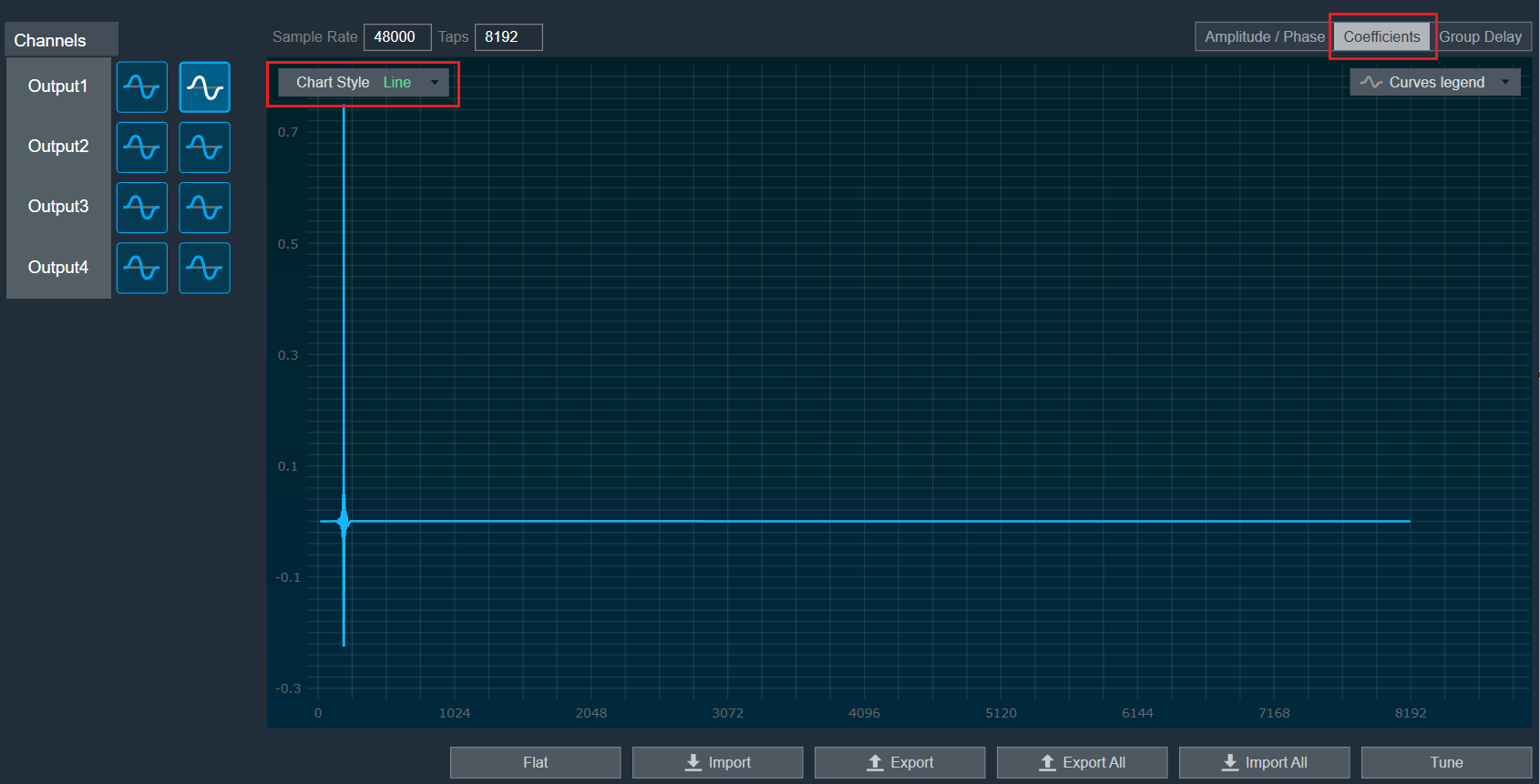 |
| Dot chart style: when “Chart Style” selected as Dot, the Coefficients graph. | 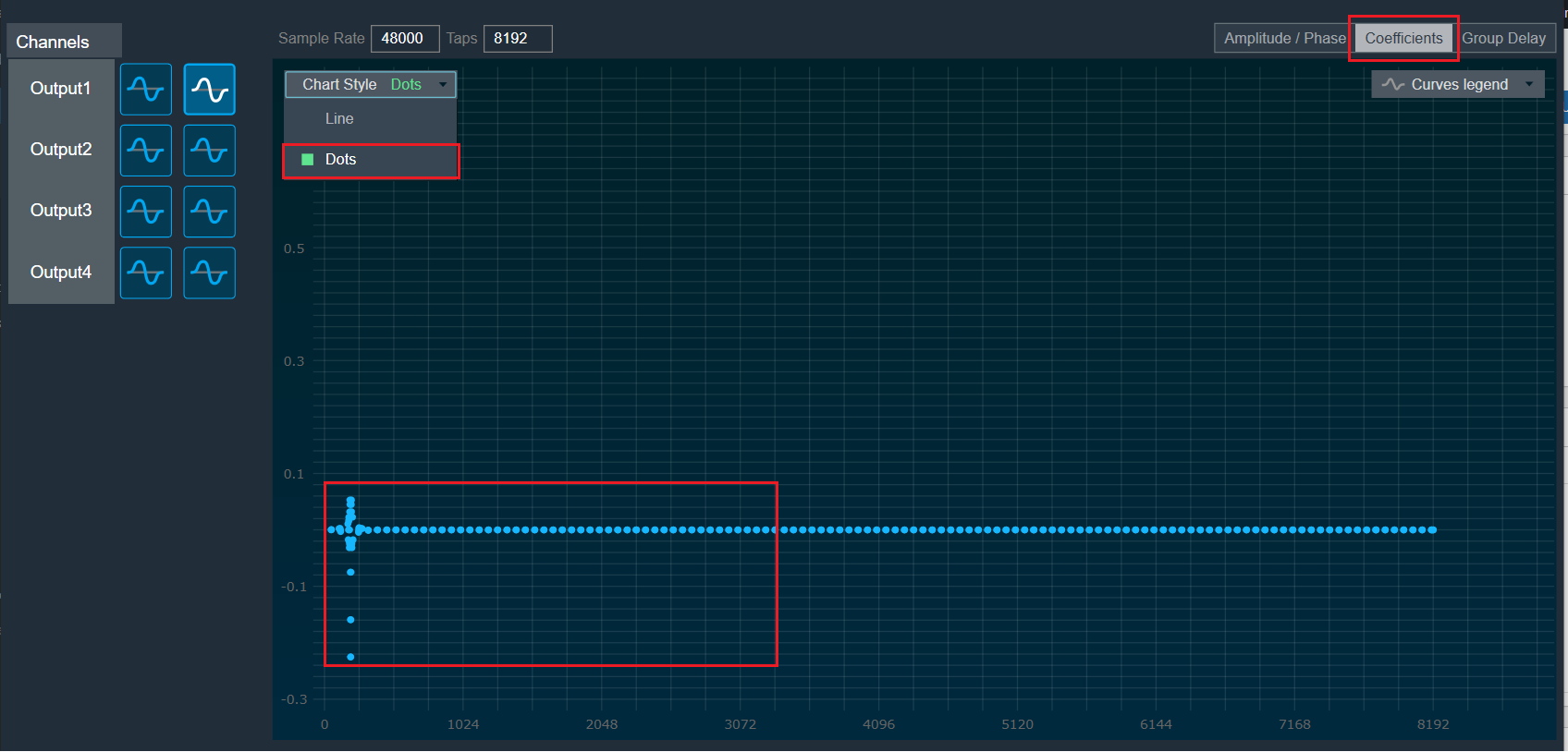 |
Group Delay: When the coefficients are given and “Group Delay” option is selected, the graph display the values.
Curves Legend: This option allows you to show the details of which graph tab (Amplitude/Phase, Coefficients, Group Delay) is selected.
| On the selection of Amplitude/Phase graph tab Curves Legend will show below information. |  |
| On the selection of Coefficients graph tab and Chart Styles ‘Dots’, Curves Legend will show below information. |  |
| On the selection of Coefficients graph tab and Chart Styles ‘Line’, Curves Legend will show information. |  |
| On the selection of Group Delay graph tab, Curves Legend will show information. |  |
Additional Functionalities
- Flat : This is used to make the graph flat by making coefficients to 0.
- Import : This function is used to import the coefficients for a single active filter. Click on the “Import” button, then enter the file path and click Ok.
All coefficients for the selected filter will be imported, as shown in the graph. If the number of coefficients does not match the number of taps, a warning pop up will appear. Click ‘Yes’ to import available coefficients or click ‘No’ to cancel the import. - Export : This option is used to export coefficients for selected active filter into csv file.
- Export All : This option is used to export all active filters in one go. Click on the “Export All” button, enter the path and file name, then click Ok. A xml file will be created which have coefficients for each active filter.
- Import All: This option is used to import all coefficients in one go. Click on the “Import All” button, enter the XML file path and then click Ok. All the given coefficients will be imported and can be seen in the graph.
- Read: This is used to read from the target to display in the panel.
- Tune: This is used to apply tune for given value.
Configure Coefficients through Virtual prediction
- On the MIMO Convolver tab, click on Measurement Coefficients. The Virtual Tuning window appears.
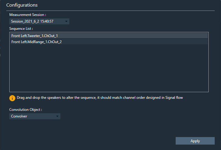
- Click Apply after selecting Measurement session from drop-down list.

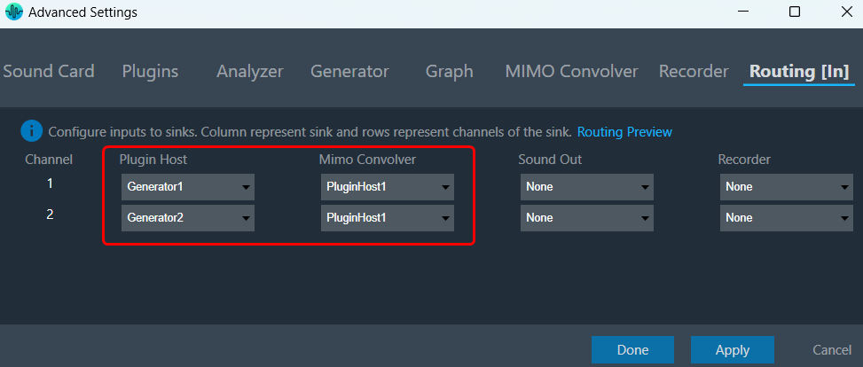
- Go to the Routing [in] tab.
- Set the inputs for “Plugin Host” (such as Generator1 and Generator2). These inputs will determine the channels from the Plugin Host that will be used.
- Set the inputs for “Mimo Convolver” in order to route the PluginHost output channels to the sound card outputs.
Example 1: PluginHost1 and PluginHost2, if output of Plugin Host is fed to MIMO Convolver.
Example 2: Generator1 and Generator2, if generator is fed to MIMO Convolver.
- Go to the Analyzer tab and select Plugin Host (MIMO convolver) output as the channel source.
- Set the Channel source (such as Generator1, PluginHost1, and MimoConvolver1) to display in chart.

- Once the settings have been updated, click Done.
- Connect to device through Plugin Host. For more details, refer to Plugin Host Setting.
- Open Channels, assign channels to Graph A and Graph B.
A chart with Genertor1, PluginHost1, and MimoConvolver1 outputs appears.
3.5.7.Recorder Settings
In RTA, the Recorder is a sink type that allows recording in mono or stereo mode, with the option to configure the number of channels to be recorded. The Recorder supports both “Append” and “Overwrite” modes and can be synchronized with the generator signal.
To configure the Recorder settings, navigate to the Recorder tab in the RTA Settings window.
The below example shows Recorder is set to 5 channels with mono mode.
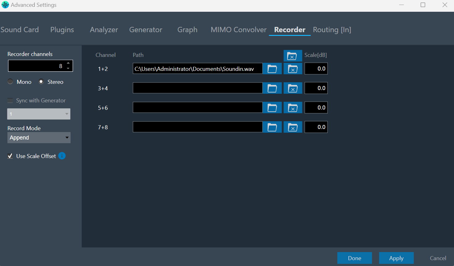
- Mono mode: 1 channel will record per file.
- Stereo mode: 2 channels will record per file. Recording can be appended to the same file or overwritten using Record mode.
- Sync with Generator: The Recorder and Generator will be in sync with this option. When the Generator starts, the recording begins automatically, and vice versa.
Choose the generator instance from the drop-down menu that is synchronized with the recorder. - Use Scale Offset: The scaling factor can be used to amplify or attenuate the recorded signal, as explained in the information tooltip. Scale offset can be set per recording channel.
When you click on the “Close” button, the selected file for the channel is removed from the tab settings and the channel is closed for recording until the settings are applied with the “Done” button.
Max supported recording channels are 64 and supported recording file format is .Wav.
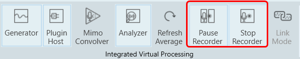
Once you have finished configuring the recorder, use Start or Stop the recorder and Pause or Resume it.
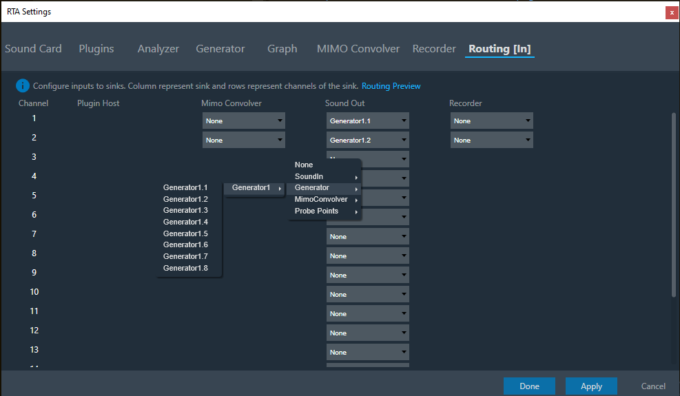
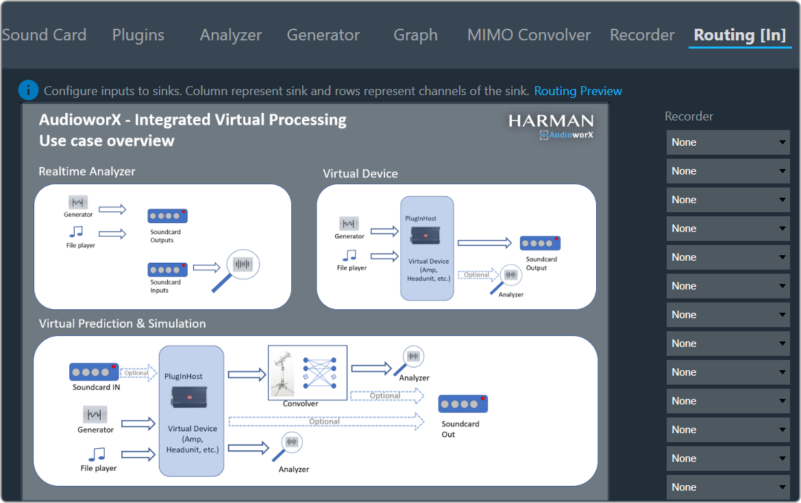
3.5.8.Routing Settings
Audio signal routing refers to the process of directing audio signals from a source to one or multiple destinations within an audio system. In audio systems, signal routing can be achieved through different methods, depending on the complexity and requirements of the setup.
On the Routing tab, the connections to the sound out devices, plugin host, mimo convolver and file recorder can be set.
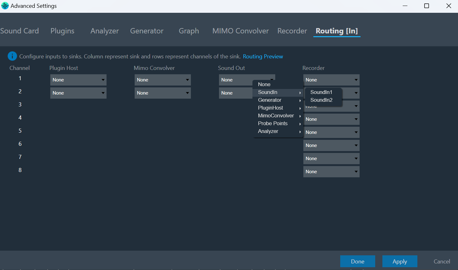
The Sound Out channels 1 to 16 correspond to the channel pairs found in the “Streams” section of the “Sound Card” settings. Click on a control in the “Sound Out” column brings up a context menu from which you can choose a source.
Currently, the player is not supported as a source.
The Analyzer channels (excluding Average channels) can be set as source for recorder to any Routing sinks. The recorded data should be same as analyzer data if Analyzer is set as source for recorder.
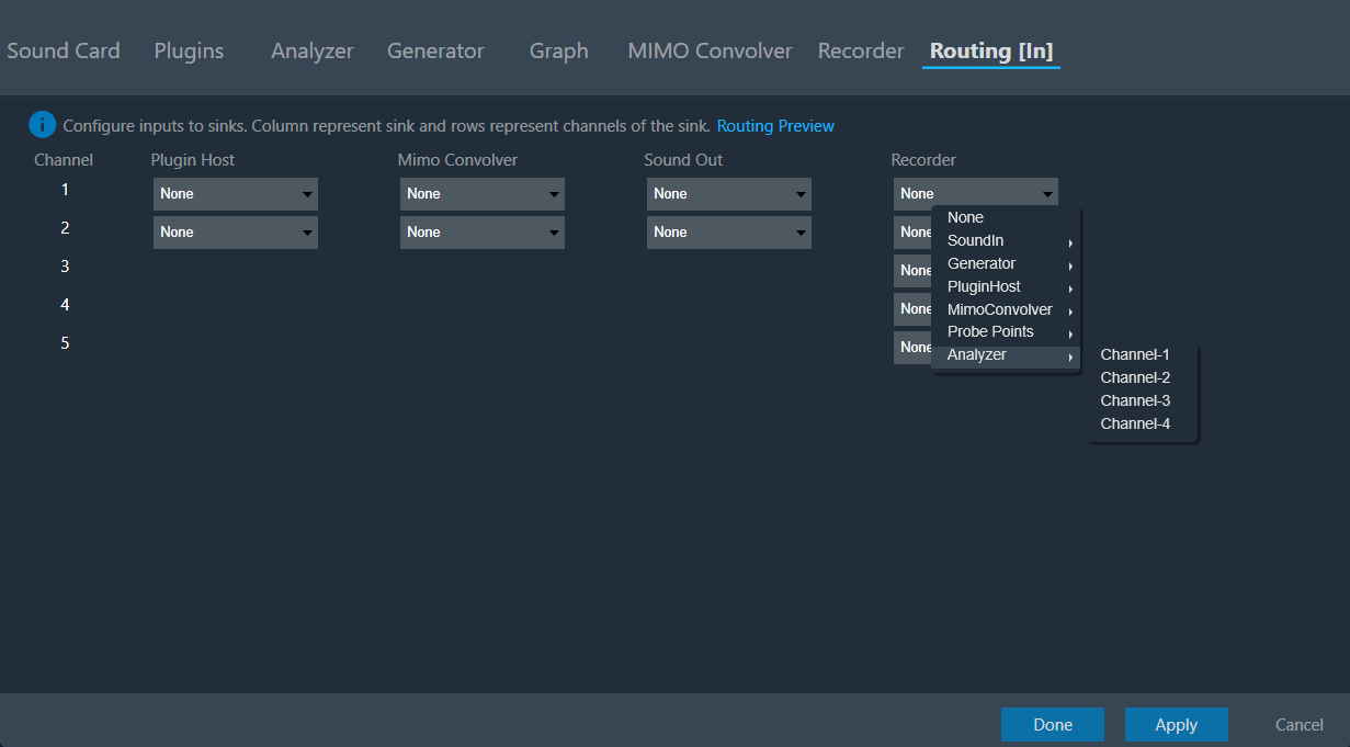
Upon clicking “Routing Preview,” a use case overview will appear to enhance the understanding of Routing.
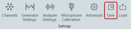
3.6.Saving RTA Settings
Once you complete all the RTA settings, click on the “Save” option. A file save dialog box will appear, enter the file name, and click Save.
Upon clicking “Save” within the dialog box, all of the following settings will be exported to a file with the. rta extension in a human-readable JSON format.
- Generator
- Analyzer
- Audio Driver
- Display
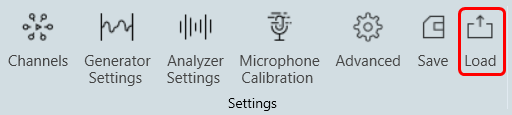
3.7.Loading RTA File
Upon clicking the “Load” button, a file open dialog box will be displayed. Locate the desired .rta file and click “Open” to restore the RTA settings stored in that file. The loaded settings will take effect immediately.
If the sound card settings are invalid when you load the settings, a settings window will be launched. You will need to fix the sound card settings issue before being able to proceed further.
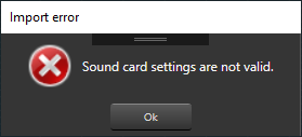
Upon clicking the “Apply” button, the sound card settings will be applied. Subsequently, you can modify other settings according to your preferences.
After importing the settings, it is necessary to reconnect the device.
4.Integrated Virtual Process (IVP)
Integrated Virtual Process (IVP) refers to the use of virtualization technology to create a seamless and interconnected environment for analyzing various audio signals processes. It involves following operations.
- Generating virtual signals
- Connecting Plugin Host
- Utilizing Mimo Convolver
- Analyzing audio signal
- Utlizing Probe Points
You can start Integrated Virtual Processing by clicking the “Analyzer” or Play button.
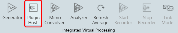
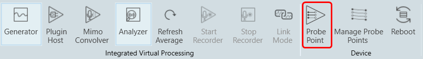
Integrated Virtual Processing is a combination of the following options.
- Generator: Used to start/stop generator.
- Plugin Host: Used to start/stop plugin host
- Mimo Convolver: Used to start/ stop mimo convolver.
- Analyzer: Used to start/ stop analyzer.
- Probe Points: the Probe Point functionality facilitates the streaming of data from any stage of the signal flow to GTT, enabling the analysis, recording, or reuse of the data within IVP.
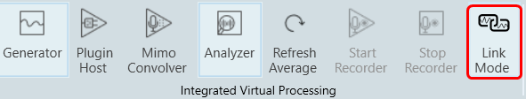
- LinkMode: The Link Mode feature allows you to establish a connection between the measurements in the upper and lower graphs on the RTA screen.
4.1.Link Mode
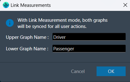
The Link Mode feature allows you to establish a connection between the measurements in the upper and lower graphs on the RTA screen. This connection enables you to perform trace capture and other operations simultaneously on both graphs.
In order to enable Link Mode, you need to configure the Analyzer settings mode option to Multiplexer.
On clicking Link Mode, you will be presented with an option to provide the name of the charts from the below window. Once the linking is activated, any operation performed on the Traces in the upper graph, will be reflected in the lower graph. The upper graph will refer to Average channel 1 and the lower graph will refer to Average channel 2.
5.Device Settings
5.1.Probe Points
The Probe Point functionality facilitates the streaming of data from any stage of the signal flow to GTT, enabling the analysis, recording, or reuse of the data within IVP. The primary purpose of this feature is to provide the capability to receive data from an audio object and perform real-time analysis of audio input using the Real-time Analyzer view.
Configure Probe Point
To enable probe points per core:
- Open the Device View and select the Virtual core layer of the device.
- Go the Virtual core properties, select the Streaming checkbox, and set a number of probe points per core.
Only the configured number of probe points can be enabled in signal flow per core.
The configured probe points will be sent to the device using the “Send Device Config” feature. This configuration can be fetched from the device using the “Load Device Config” feature.
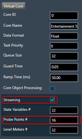
In order to utilize streaming for state variables, it is necessary to enable this feature. However, considering its resource-intensive nature, this high configuration feature can be skipped to ensure optimal utilization of MIPS and memory. The count of probe points specifically pertains to audio streams and maximum 16 probe points are supported for a core.
If Streaming is disabled for the core, the number of probe points input field will be disabled and streamable state variables will be excluded for that core in the streaming window.
Add Probe Point
Probe Point context menu for selected connection has the below options:
- Add: The feature allows you to add a probe point on a selected connection source point. Additionally, the default state of the probe point is set to the enabled state.
To add probe point on the virtual connection:
- Right-click on the virtual connection > Probe Point > select Add.
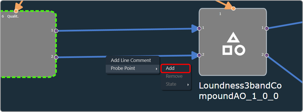
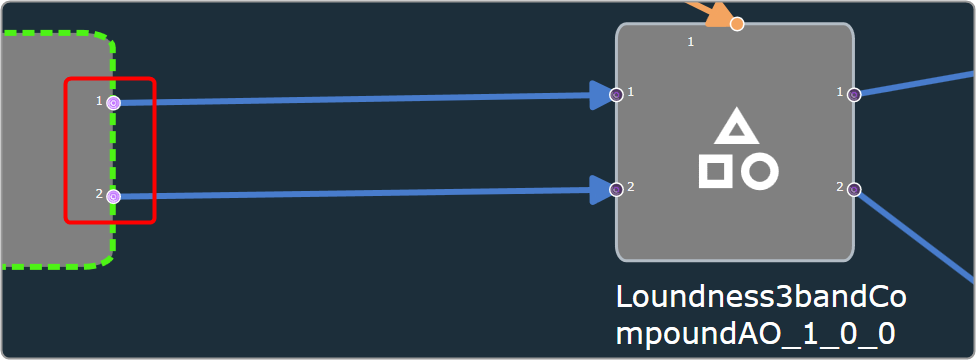
After adding probe points, the source point pin connection will be visually highlighted with a bright purple-colored icon.
Remove Probe Point
- Remove: You can remove a probe point from the selected connection.
To remove probe point from the virtual connection:
- Right-click on the virtual connection > Probe Point > select Remove.

- State: You can alter the state of probe point on a selected connection.

| Enable | Change probe pin state to enable and pin will be highlighted with bright purple colour icon. |
| Disable | Change probe pin state to disable and pin will be highlighted with grey dark purple colour icon. |

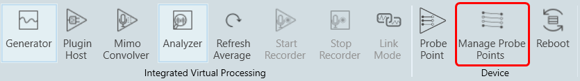
5.2.Manage Probe points
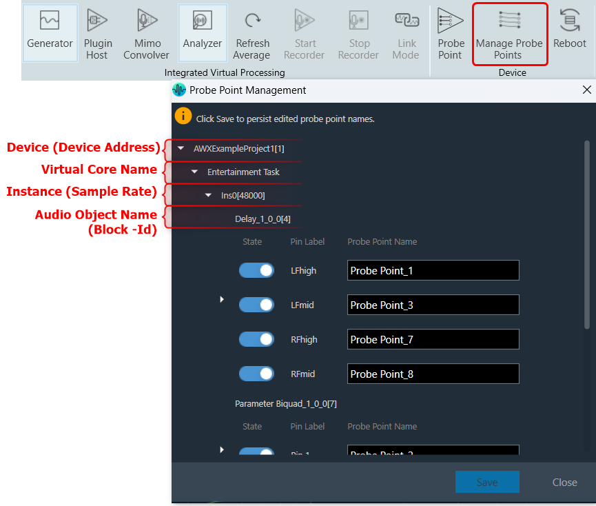
Open Probe point management window through ‘Manage probe Points’ ribbon button.
The Manage Probe Points allows you to enable or disable probe point and edit probe point name in the Probe Point Management window.
In the Probe Point Management window, the probe points are organized in the following order.
- Device [Device address]
- Virtual Core name
- Instance [Sample Rate]
- Audio Object Name [Block- Id]
Additionally, State, Pin Label and Probe point name is displayed for each probe point.
This window will consistently stay synchronized with the probe point states in the Signal Flow Designer.
After making all the necessary modifications, click Save to persist edited probe point names.
Configure probe points in RTA/IVP
- Open Advanced Settings window
- Select Probe Points as Analyzer / Recorder / Sound out sources.
- Click Done.

To record the probe point signal.

Start Probe Point Streaming
Pre-requisites:
- Make sure to enable the Probe Point feature for the core.
- Ensure that the number of active probe points is set correctly.
- Ensure that the Probe Points used in the IVP configuration are correctly configured as a source (Analyzer, Recorder, etc).
- Start Plugin Host and establish connection with device.
Use IVP Block Length <= 512 for probing to avoid frame dropping.
Once you have configured as per the above pre-requisites, click on the Probe Point to start.
Example of Streamed data.
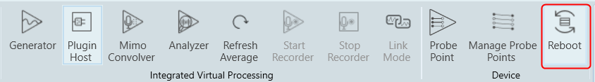
5.3.Reboot
When you click on a “Reboot” button, the device will restart. During the reboot process, the plugin host will go through a shutdown sequence and then start up again.
After the reboot, the plugin host will return to its previous state.
6.Real Time Data View
The ribbon bar provides a quick view of real-time measurements for RMS, THD, True Peak, Peak-Frequency, and THD+N. By default, the tool selects two channels for this display and you can view the live data of two channels simultaneously. If you want to monitor a different channel, you can easily select it from the options available on the ribbon bar.
When using a multiplexer, it will load average channels by default; otherwise, it will peak the first channels that are listed on the analyzer.
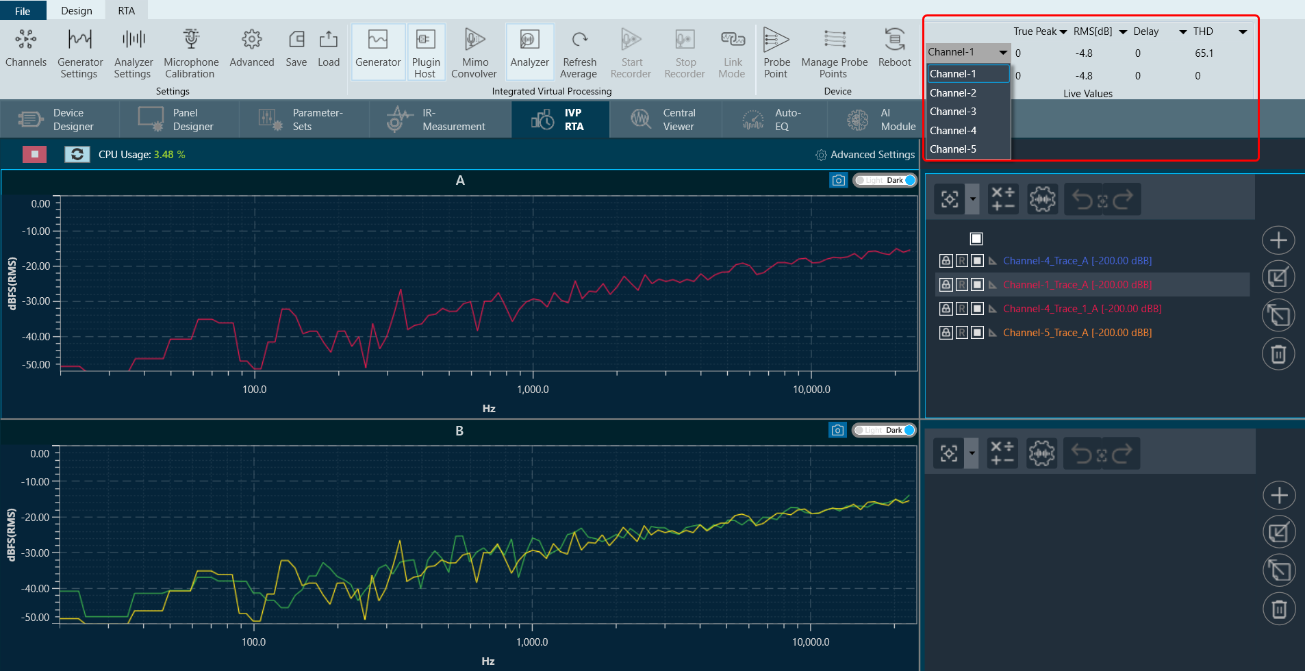
RMS Values will provide the selected weighting indication (A B C).
The Weighting is displayed on the ribbon bar when configured in Advanced Settings. Go to Advanced Settings > Analyzer > Freq Weight RMS to activate weighting.
There are four live data columns available for selection:
- RMS
- THD
- True Peak
- Peak-Frequency
- THD+N
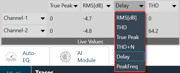
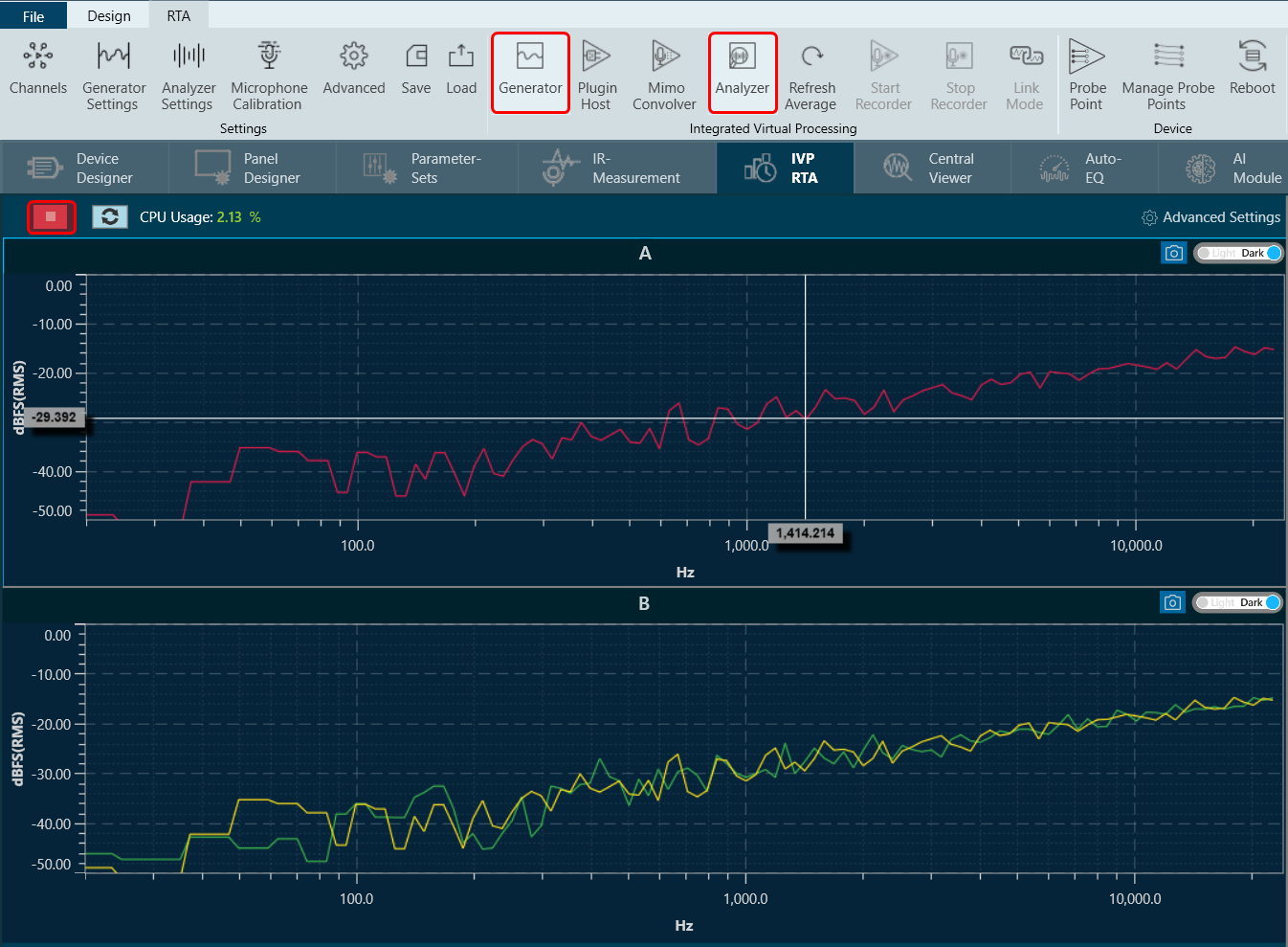
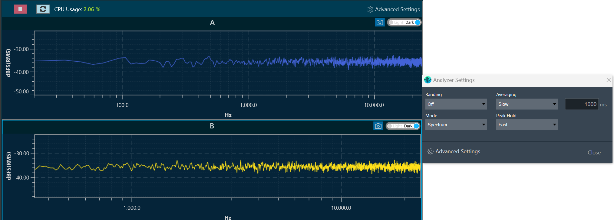
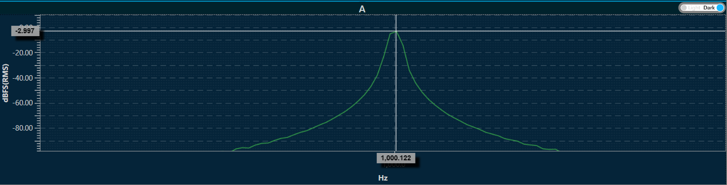
For example, for the 1 kHz sine wave, the live ribbon and graph will look as follows:

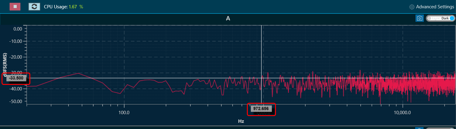
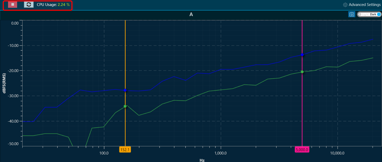
CPU Load
In the RTA graph view, the CPU load provided by Audio Engine is displayed in percentage (up to 2 decimal). This will be shown in different colors based on the level as below.
- Normal: 0-70 (Green color)
- Medium: 71-95 (Yellow color)
- High: Greater than 96 (Red color)
7.Graph Settings and Measurement
Cursor Measurement
When hovering the mouse over any of the curves or plots on the graph, the horizontal and vertical values of the X and Y positions pointed to will be displayed. It is important to note that while the X value will follow the mouse pointer, the Y value will show the value of the closest trace.
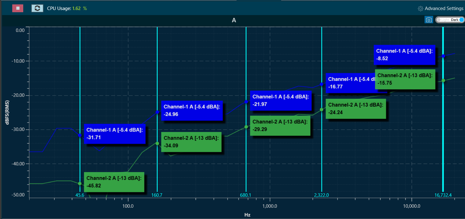
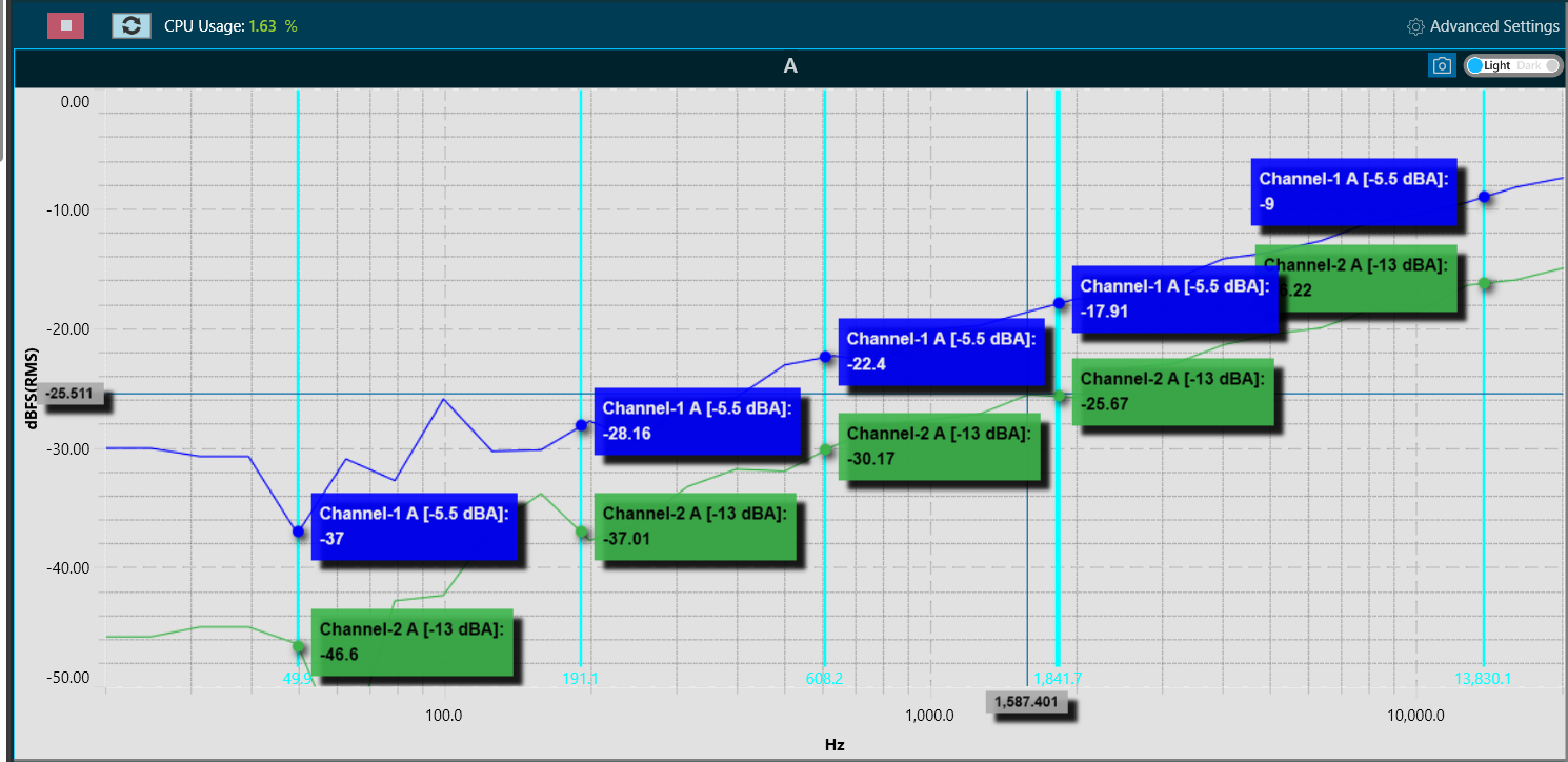
Add Marker
You can mark the curves for value inspection. Press CTRL + click, to create a marker. This marker will display the values of the traces as tooltips on top of the charts. It will show the values of all the traces.
A maximum of 5 markers can be placed on the chart.
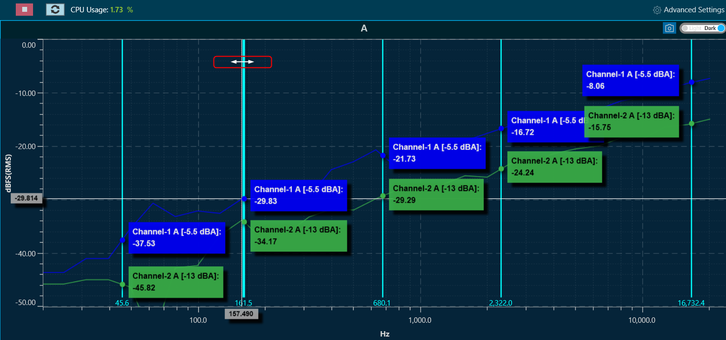
To remove a marker, select the marker by clicking on top of it. The line of the marker will become wider, indicating it has been selected.
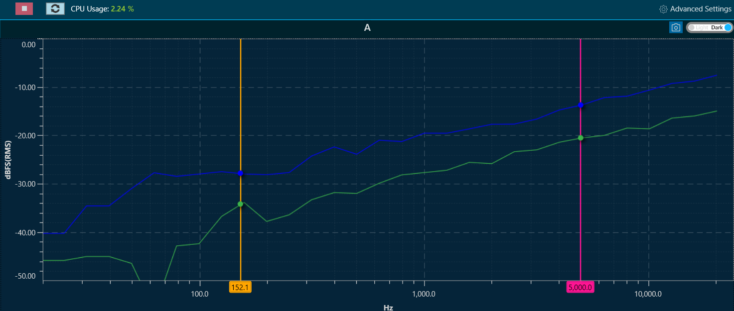
Add Delta Marker
Delta marker helpful in creating differential values for selected curves.
To add delta markers, press ALT + click on chart, and enable measurements from traces where delta values are desired.
The selected traces will display the following information:
- The value at the first marker.
- The value at the second marker.
- The delta (difference) between the markers.
The values are indicated by the trace colour and highlighted with the marker colour. Delta markers can be dragged to the desired X position.
To disable Delta markers, press ALT + Click again.
Refresh Spectrum
In the spectrum and multiplexer modes, the spectrum refresh button will update all curves displayed, excluding the traces. This functionality allows for the resetting of averaging time periods, which is particularly significant for “forever” averaging.
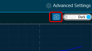
Capture Graph Image
The Export Image feature allows you to export the graphs and certain other details based on export setting configuration. The exported image file will be available in .png or .jpeg format.
Once you click on the “Export to Image” option, export setting window for the image will open.
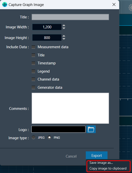
This export setting window includes following options:
- Title – Enter the image name.
- Image Width – Change the image width.
- Image Height – Change the image height.
- Include Data – Select the option to add various type of data such as Measurement data, Title, Timestamp, Legend, Channel data, Generator data in the image.
- Comments – Enter the specific comment, that you want to be add in the image.
- Logo – Add the desired logo in the image.
- Image type – Select the image type JPEG or PNG.
Once you configured export settings, click Export button. The context menu will show you two options, export the image or copy to the clipboard.
- Save image as – option will be opened to save the image to a file.
- Copy image to clipboard – will allow you to paste the graph image somewhere else.
Not possible to copy image to clipboard for graph B in case of link mode.
The exported image will have following sections based on export setting window configuration.
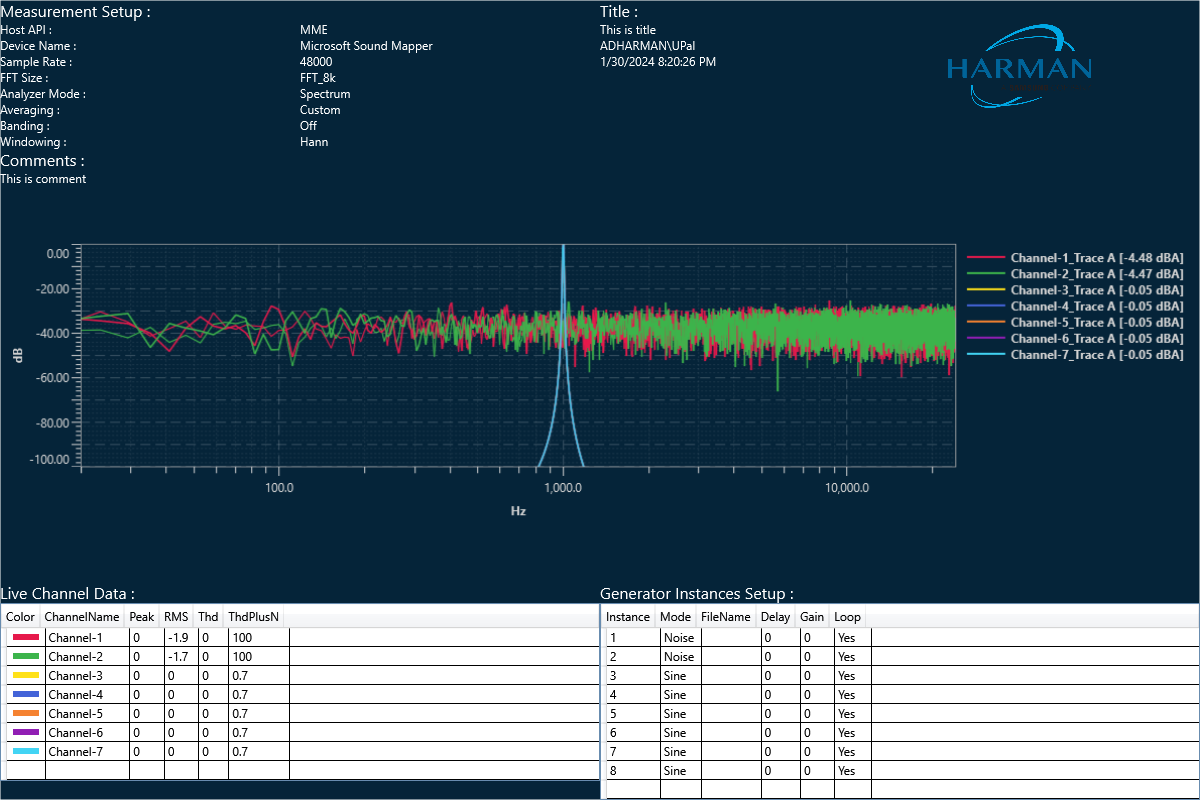
The graph always present in the exported image. Based on the export setting configuration additional sections like – Measurement information, Title, Time, User details, Logo provided, Live channel data, Generator instances details also present in the exported image .
If you select the “Channel data” checkbox, then in the “Legend” live channel entries will not appear, only traces will appear. Otherwise, all items will appear in Legend.
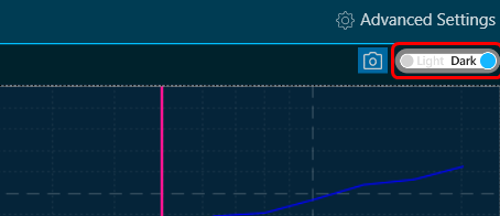
Graph Theme
There is a Toggle button (dark / light theme) in the charts in RTA graph. Once the Toggle button is clicked, the corresponding custom theme can be selected, and the background of the graph gets changed and vice versa.
|
Dark Theam
|
|
Light Theam
|
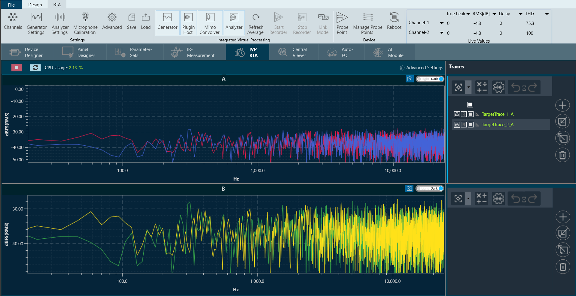
8.Traces
Traces allows you to display multiple captures of measurement curves on a single plot, allowing for quick and convenient comparisons of the measurements. The controls for traces are located on the right side of the spectrum graph.
A trace in RTA is a captured measurement curve.
There are six different kinds of traces:
- Spectrum: Complete data set from measurement without phase.
- Phase: Complete data set from measurement with phase data.
- Txt: Data imported from a text file (tab separated frequency – spectrum value pairs per line)
- Ovl: Data imported from an Overlay file format.
- Eq: Target curve, a spectrum curve described by biquad filter parameters.
- Peak Hold: Peak hold trace with three-time constants.
Traces view is available only in Frequency Domain analyzer modes like Spectrum, Phase i.e. it is not available in Time Domain.
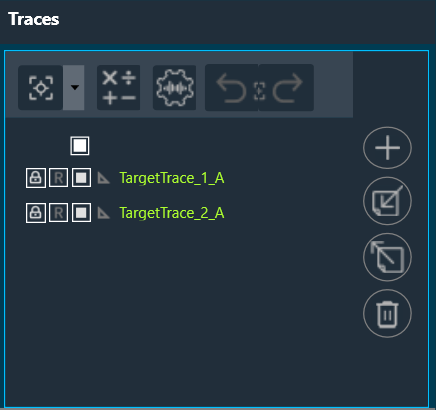
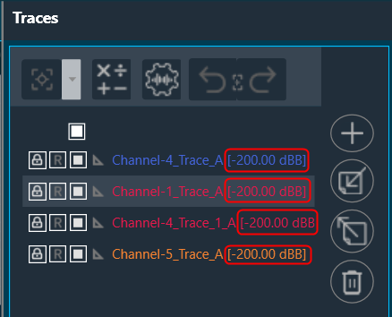
The trace menu is comprised of a trace toolbar and a trace list.
Each entry in the trace list includes a button for re-capturing, a checkbox for selection, and a trace label. The selection checkbox is used to designate the trace for mathematical operations.
Double-click on the trace label opens the trace property dialogue.
In this dialog, you can set the name, offset, and color for each trace. You can view all SPL (ABC) values simultaneously, which will aid in final documentation purposes. Additionally, “Next” and “Back” buttons are provided, allowing you to navigate through multiple traces and make edits to them simultaneously.
If you select SPL Weighting in the trace settings, you can choose to display it on the trace list without affecting the graph or live value measurements.
8.1.Trace Toolbar
The Trace Toolbar consists of several functions.
| Function | Icon | Details |
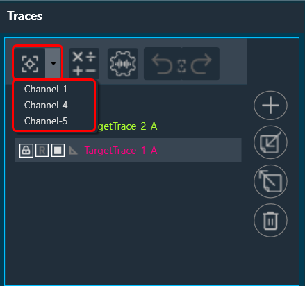
| Capture Traces |  |
The Capture Traces function provides two options:
|
| Add Math Operation |  |
The Add Math Operation allows you to generate an unweighted average, a difference, or a sum trace from the selected traces using a drop-down menu, you can identify the new traces with the green square.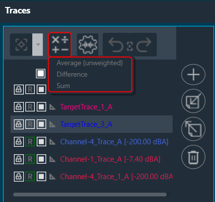 |
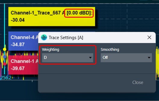
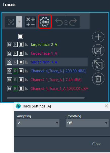
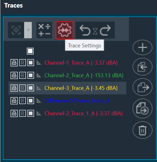
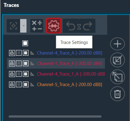
| Trace Settings |  |
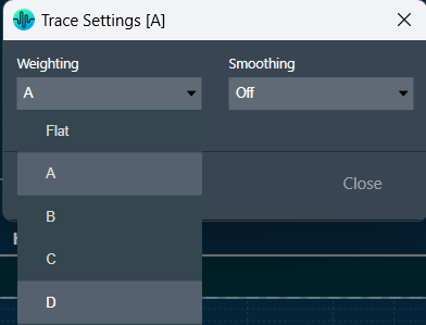
The Trace Settings allows you to configure Weighting and Smoothing functionality.
|
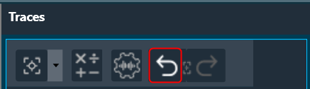
| Undo Capture Traces |
Click on the Undo Capture Traces, to reverse the last captured traces upto 3 traces.
|
|
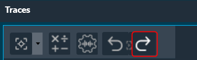
| Redo Capture Traces |  |
Click on the Redo Capture Traces, to redo the last captured traces upto 3 traces.
|
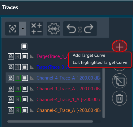
| Add Target Curve |  |
The Add Target Curve function allows you to add target curve and edit highlighted target curve using a drop-down menu.
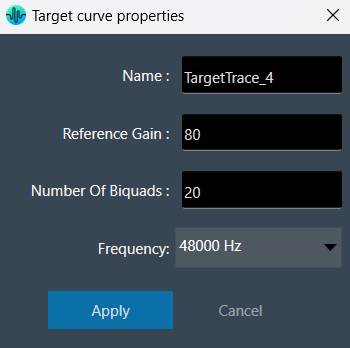
To add a target curve, click on the “Add Target Curve” option. In the target curve properties window, enter the desired curve properties, such as its name, reference gain, number of biquads and select the frequency for the target curve from drop-down. Then, click “Apply” to add the target curve.
Once target curve is active, its offset will change by 3 dB for every jump on octave banding configuration, to follow the behavior of the energetic sum of the octave banding.
To edit the target curve, click on the “Edit Highlighted Target Curve”. In the target curve properties window, change target curve properties and click “Apply”. This opens Design Target Cure window, open the Biquads on Apply to update the filters ,import and export the filters. |
| Import Traces |  |
The Import function allows you to import single traces (*.trace) or multiple traces (*.trclist) using a drop-down menu.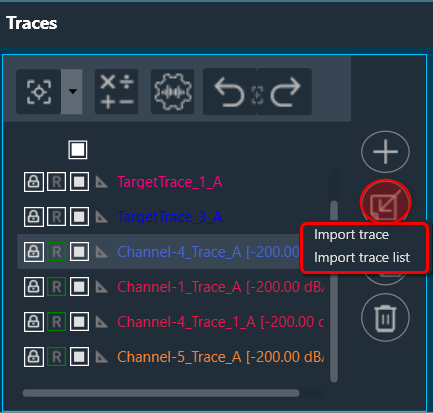 |
| Export Traces |  |
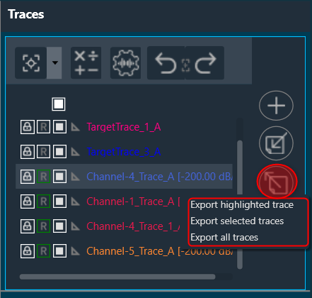
The Export function allows you to export the highlighted trace (*.trace, *.txt), selected traces or all traces (*.trclist, *.trcTxtlist) using a drop-down menu. The TraceList file can be exported as a .zip file with a (*.trace, *.txt, *.trclist, *.trcTxtlist) file extension. You can unzip the .zip file and access the individual traces from it. The exported file contains the settings details in the text file (sample rate, FFT size, Unit in column title etc) used during the capture, along with the data captured. Checked status is not retained for the tracelist exported in .txt format. |
| Delete Traces |  |
The Delete function allows you to delete the highlighted trace, selected traces, all traces, and unprotected traces using drop-down menu.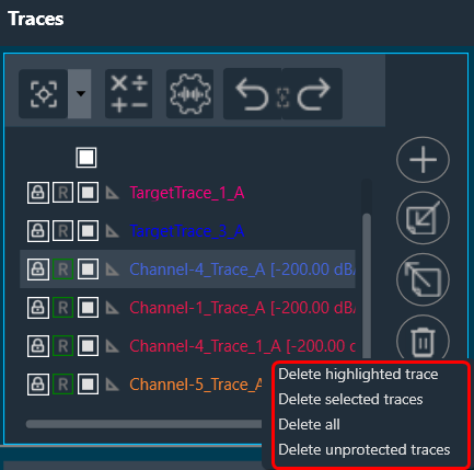 |
8.2.Trace Configuration
Enabling Peak Hold Trace
The Peak Hold Trace can be activated using a checkbox in the Advanced Analyzer menu. It’s time constants Forever, Slow, Fast can be selected in the normal Analyzer Settings Menu. The peak hold trace is reset by choosing Delete for the corresponding trace in the trace list.
To activate the Peak Hold Trace:
- Open the Advanced Settings, and enable Peak Trace feature on the Analyzer tab.

You need to enable a checkbox located in the “Advanced Analyzer” setting.
Setting Time Constants
You can configure desired time constants for the Peak Hold Trace, such as “Forever,” “Slow,” or “Fast” in the Analyzer Settings window.
If you wish to reset the Peak Hold Trace, you can choose the “Delete” option for the corresponding trace in the trace list.
Weighting on Captured Traces
The A-weighting, B-weighting, C-weighting and D-weighting are different frequency weightings that simulate how sensitive various frequencies are to the human ear.
- A-weighting (dB(A)): A-weighting is used to approximate the sensitivity of the human ear to different frequencies at low sound pressure levels. It reduces the contribution of low and high frequencies to better represent the way humans perceive sound in relatively quiet environments. A-weighted measurements are often used in assessing environmental noise levels and evaluating noise exposure limits for occupational health and safety.
- B-weighting (dB(B)): B-weighting is rarely used and has limited practical application. It was initially intended to approximate the ear’s sensitivity at moderate sound pressure levels, but it didn’t gain widespread acceptance due to certain limitations. A-weighting has largely taken the place of B-weighting in modern applications..
- C-weighting (dB(C)): C-weighting is used to measure the overall sound pressure level without any frequency weighting. It includes the entire audible frequency range and does not attenuate any specific frequencies. C-weighted measurements are commonly employed in situations where a flat frequency response is desired or when assessing high-level noise sources, such as loudspeakers or industrial machinery.
- D-weighting(dB(D)): D Weighting is used to measure sound pressure levels with a frequency weighting that is specifically designed to reflect the human ear’s sensitivity to loud noises, particularly in the presence of high-level aircraft noise. Unlike C-weighting, D-weighting emphasizes certain frequency ranges to better correlate with the subjective perception of aircraft noise.
Weighting feature is used to adjust measurements to better align with the perceived loudness by human listeners.
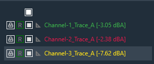
When you select the “Trace Settings” option in the Traces toolbar, a new window will open, allowing you to choose the desired Weighting (Flat/Unweighted, A, B, C, and D).
Based on desired selection weighting will be applied to all captured traces. Each trace RMS SPL value will be displayed in traces view as shown below.
Trace Properties
All capture traces can be modified double clicking over them:
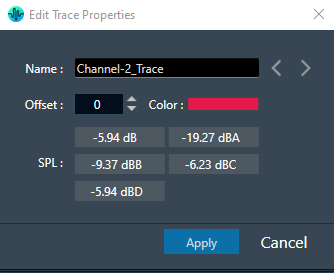
In the context menu could be find the capability to update the name, set the offset, set the color and see the different weighting values (A, B, C, D).
Smoothing on Captured Traces
Smoothing is a technique that reduces variations in plotted curves to improve the visual perception of trends or patterns in frequency response or level measurements. It is commonly used in audio analysis and equalization tasks to enhance clarity while considering the trade-off between noise reduction and preservation of important details.
When you select the “Trace Settings” option in the Traces toolbar, a new window will open, where you can select desired octave banding for smoothing. Based on desired selection smoothing will be applied to all captured traces.
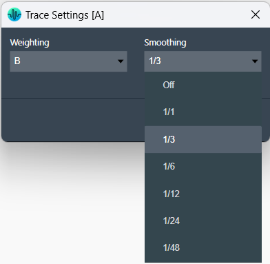
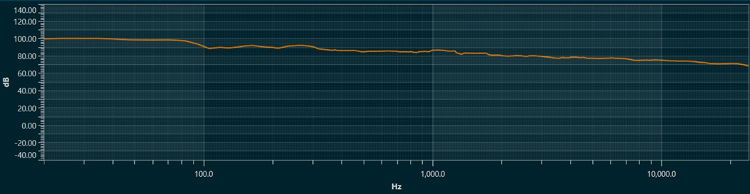
The smoothed curve with the chosen option looks like below figure.
8.3.Select/ Deselect All Traces
Select/ Deselect All Traces
At the top of the Traces view, there is a checkbox that enables you to either select or deselect all traces. When you select the checkbox at the top, all traces within the trace window will be automatically selected. Similarly, when the top checkbox is deselected, it will unselect all the traces in the trace window.

When the top checkbox in the upper trace window is selected in linking mode, it automatically selects all the traces from both the upper and lower trace windows. Similarly, when the top checkbox in the upper trace window is unselected, it will unselect all the traces from both the upper and lower trace windows.

Lock / Unlock Traces
When the trace is locked, the recapture on that trace is disabled. Once unlocked the trace can be recaptured. This button toggles between locked and unlocked states.

Recapture Traces
The trace can be recaptured from the signal for the same channel using this option.

Select / Unselect Trace
The trace can be made visible and hidden on the graph using this option.

Show Measurement
The measurements can be shown on the graph for the trace using this option.

8.4.RTA Shortcuts
The RTA shortcut keys allow you to perform quick action using keyboard keys. Various shortcuts are implemented in the RTA module to increase efficiency and facilitate easy navigation. These shortcuts provide quick access to frequently used functions within the GTT.
You cannot open multiple windows using a shortcut.
The table below provides you detail about available shortcuts in RTA module.
| Shortcuts keys | Operation | Shortcuts keys | Operation |
| F2 | Channels Quick Settings window. | Ctrl+Delete | Delete selected (highlighted) trace of highlighted chart. |
| F3 | Generator Quick Settings window. | Ctrl+Shift+Delete | Delete all traces of highlighted chart. |
| F4 | Analyzer Quick Settings window. | Alt+A | Switches between Averaging Mode. |
| F6 | Microphone Calibration window . | Alt+G | Start/Stop Generator. |
| F7 | Export Settings Window Dialog. | Alt+M | Multiplexer Mode (Average). |
| F8 | Import Settings Window Dialog. | Alt+O | Switch between Banding Mode. |
| F9 | RTA Advanced Settings window. | Alt+R | Refresh average values. |
| Ctrl+C | Perform Capture Trace action into the traces panel of highlighted chart. | Ctrl+A | Hide all traces of traces panel of highlighted chart. |
| Ctrl+E | Export selected (highlighted) trace of highlighted chart. | Ctrl+Shift+E | Export All Traces of highlighted chart. |
| Ctrl+I | Import Trace into the traces panel of highlighted chart. | Ctrl+H | Hide selected (highlighted trace) of highlighted chart. |
| Ctrl+Shift+C | Recapture action of selected (highlighted) trace of highlighted chart. | Spacebar | Start/Stop Analyzer. |
| Ctrl+Shift+I | Import List Trace into the traces panel of highlighted chart. | ESC | Close Floatable window. |
Zoom and Scroll Controls
The following controls can be used to perform zoom and scroll functions on the graph.
| Alt + MW (Zoom on Y axis) | Expand the Y axis to zoom in or out of the values on the graph. |
| Ctrl + MW (Zoom on X axis) | Expand the Y axis to zoom in or out of the values on the graph. |
| Shift + MW (Scroll on X axis) | Scroll the visible graph along the X axis up to the visible or configured limits, that is, if the graph shows the maximum visible value in the configured X, the scroll will not be available. |
| MW (Scroll on X axis) | Scroll the visible graph along the Y axis up to the visible or configured limits, that is, if the graph shows the maximum visible value in the configured Y, the scroll will not be available. |
MW=Mouse Wheel
9.Analysing Audio Signal
Configure Basic Measurement
Steps to configure basic measurement for analyzing audio signal.
- On the IVP RTA tab, click on the Advanced or Advanced Settings. This opens RTA Settings window.
- On the RTA Setting window, select the Sound Card tab, and then select the “Sound In device” that is connected to a microphone for channel 1 + 2.
- Switch to the Analyzer tab, click on the Source for Channel-1, and select SoundIn1 from the context menu.
- When you have finished configuration, click Done to close the Setting dialogue box.
- On the ribbon bar, click on Analyzer. The RTA graph now displays the incoming microphone signal in the time domain.
- In order to display the spectrum of the signal, click on the Analyzer Settings in the ribbon bar. This opens the Analyzer Setting window.
- On the Analyzer Settings window, set the Mode to Spectrum from the drop-down list.
The graph now displays the spectrum of the incoming microphone signal.
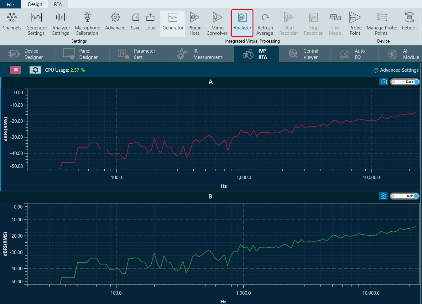
As only one channel is active, the lower graph has been minimized by dragging the middle line and placing it at the bottom of the window.
Analyse RTA without Soundcard Signal
In order to test RTA without a soundcard signal, the test signal generator can be connected directly to the analyzer.
- On the Analyzer Settings window, click on Advanced Settings. This opens RTA Settings window.
- On Analyzer tab, click on the “Source” for Channel-1, and select Generator 1 from the context menu.

- When you have finished configuration, click Done to close the Setting dialogue box.
- On the ribbon bar, click on Generator, and click on Analyzer or “Play” button. The RTA graph now displays the spectrum of a 1 kHz sine signal.