User Guide GTT Legacy Viewer

The measurement functionality has been removed from the Legacy Measurement Module with S-release. Since then, this module is used for measurement data management and viewer purposes and is called Legacy Viewer. The currently active parts are described in this documentation.

The Legacy Viewer user interface is started by selecting the Legacy Viewer in the ribbon bar of the GTT main window (red circle). If the Legacy Viewer has been launched successfully its status can be checked by opening the services monitor (green circle).
This will present all services used by GTT and their status.

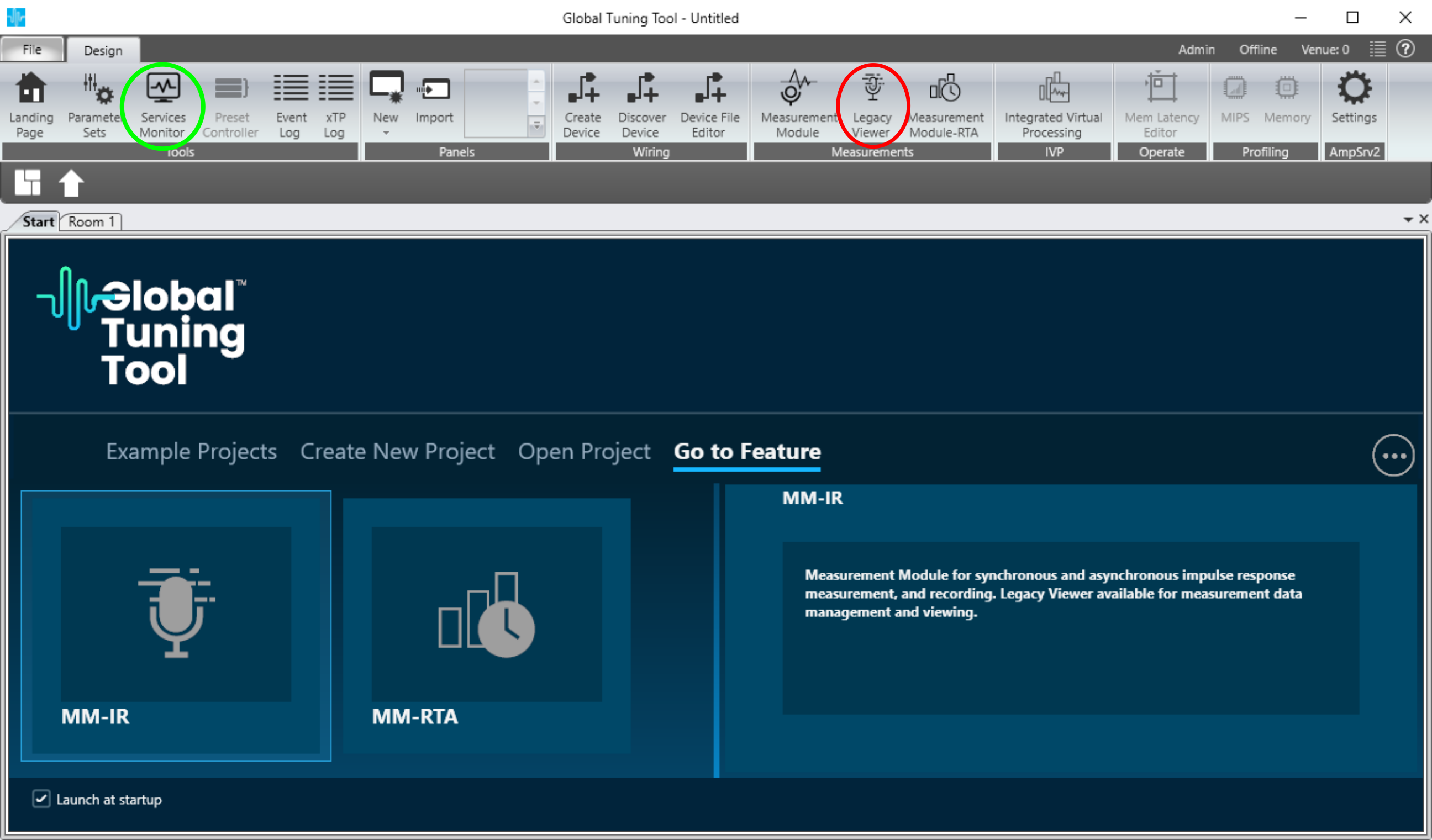
The Legacy Viewer will open as a new tab in the main GTT window.

Available measurements can be grouped and selected for being viewed. The right area allows to delete measurements (4) and view the results (5). In the middle area, if any of the sessions appear with a warning icon this indicates that session raw data is missing, it can be re-linked with (1). Sessions can be exported in readable format (json) (6), raw measurements can be imported/exported to/from the project (2 and 3). If one of the above buttons is disabled (greyed-out) it means that a prerequisite hasn’t been met.

The next paragraphs follow the numeration in the figure above.

The main window allows to reorder and filter the measurement in a very straightforward way:

Reordering, by dragging and drop the filter bar, the organization of data change accordingly.

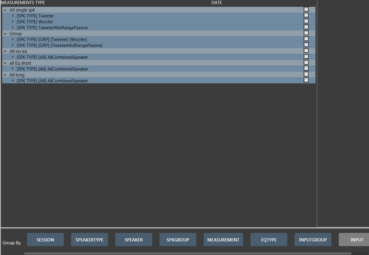
Organized by session.

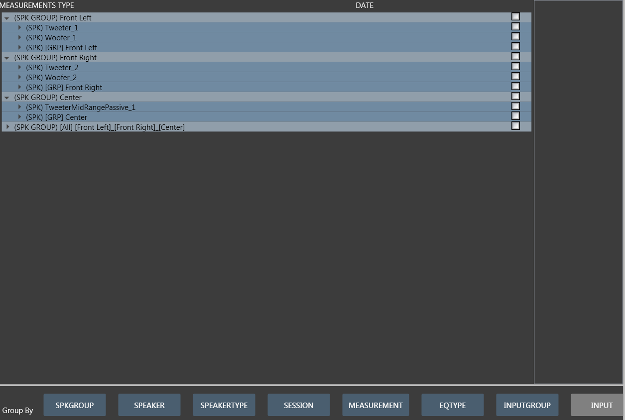
Organized by speaker group.

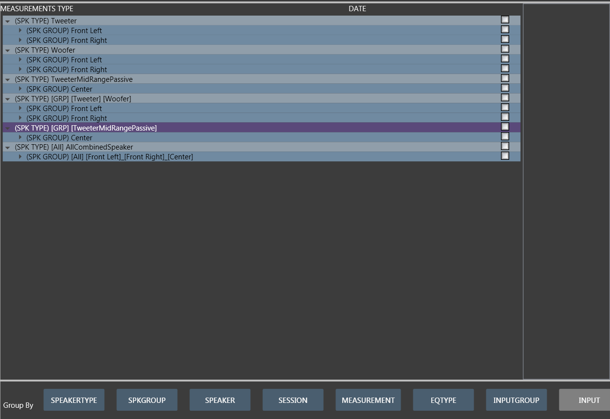
Organized by speaker type.

All the measurements Time response and Frequency responses can be analyzed using Run Viewer option (button 5).

The viewer interface looks as follows

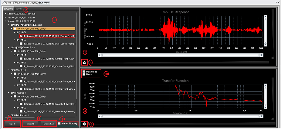
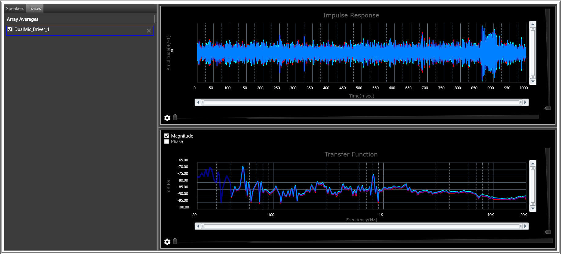
All selected measurement sessions will be listed in a tree view structure (1) , all generated Averages will be listed in the traces tab (2) , selected microphones and average curves, impulse responses and transfer functions will be plotted in graph (3 and 4) . Impulse response and transfer function parameters can be modified (5 and 6) , magnitude and phase plotting can be enabled/disabled(10) , selected sessions can be exported in readable format (7) , all sessions can be selected/deselected with one click using select/deselect buttons (8) . The plot settings for graphs can be inhibited using inhibit plotting checkbox (9)

Within the impulse response viewer is possible to modify some parameters to improve the presentation of the IR and the relative transfer function. Click on the settings icon of the relative chart.

For the Impulse response, it is possible to cut the IR and window it.

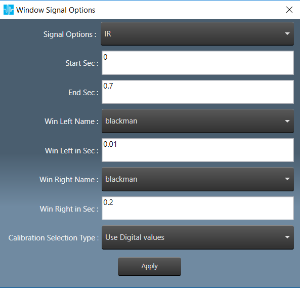
• start, in seconds.  The start cut of the IR
• end, in seconds.  The end cut of the IR
• Win Left Name, the window applied to the left side of the cut (see image below)
• Win Left in Sec, the length of the left side window in seconds
• Win Right Name, the window applied to the right  side of the cut
• Win Right in Sec, the length of the right side window in seconds
• Calibration Selection type
  For IR three types of calibration, accordingly to hats manual, p.39
  1. Digital Values: the compensation constant are not considered, the results and the units are in a.u. (arbitrary unit)
     HATS equivalent Transfer Function v/v (small v doesn’t stand for volt!).
     In MM this is called arbitrary unit a.u. and it is displayed as dBFS
  2. Arbitrary OUTPUT calibration (output calibration not yet implemented in GTT) as a workaround for proper Units in Transfer Function  (H(f)) (0dBFS → 1Vpk)
     HATS equivalent, Normalized Sound Pressure Level Pa/V
  3. Calibration (removed stimulus), (Hpa(f)) to have a PASCAL outcome, independent from the generator
     HATS equivalent, Sound Pressure Level Pa

   

  

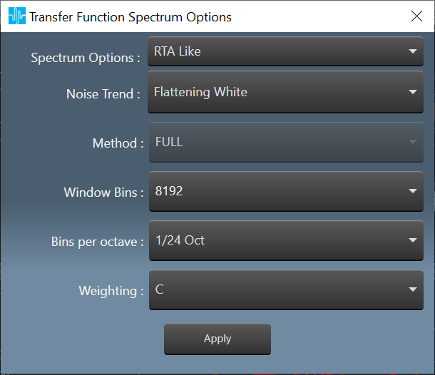
The Transfer function options in the Frequency domain allows displaying the IR as transfer function in the complex frequency domain (magnitude+phase). Two methods are implemented:

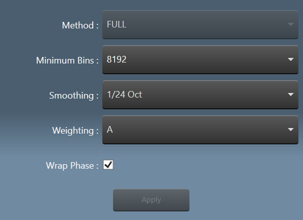
• Method, now is fixed to FULL (welch is deactivated and selected automatically for recordings).
• FULL the power spectrum, or single-sided auto-spectrum, contains the squared RMS amplitudes of the signal. The signal cut and the windows selected in the time domain (see above) is fully transformed and its Power density calculated. There are no options, the frequency array is automatically computed, based on the next power of 2 of the IR length for an FFT, the frequency bins are calculated accordingly. This method also provides the phase of the TF
  It is also possible to select the smoothing for spectrum and phase. Pressing apply will update the chart.

• Minimum bins, the minimum number of bins of the FFT. If the signal is larger of minimum bins an FFT zero-padded to the next power of 2 is computed.
• Smoothing of spectrum and phase
• Weighting is used to emphasize or suppress some aspects of a phenomenon compared to others, for measurement

• Wrap phase: if selected, limit the phase in the range -180/180 degree.
  

• WELCH (DEACTIVATED FOR END USER), computes an estimate of the power spectral density by dividing the data into overlapping segments, computing a modified periodogram for each segment and averaging the periodograms.
  This method doesn’t provide the phase of the TF (a zero vector is generated instead)
  P. Welch, “The use of the fast Fourier transform for the estimation of power spectra: A method based on time averaging over short, modified periodograms”, IEEE Trans. Audio Electroacoust. vol. 15, pp. 70-73, 1967.
  

• BINS per segment, number of points used to calculate the FFT of every segment in WELCH
  Segment Overlap, Percent of Bins per segment to overlap between segments
• Segment Window, the window used for conditioning every segment

With the viewer it is possible to inspect and analyze the recording as well

• select Recorded as signal type, length and windowing works as usual but are applied to the recording
• 
• Two possible spectrum processings are available for recorded signals
  • • The Usual Power Spectrum
    • 
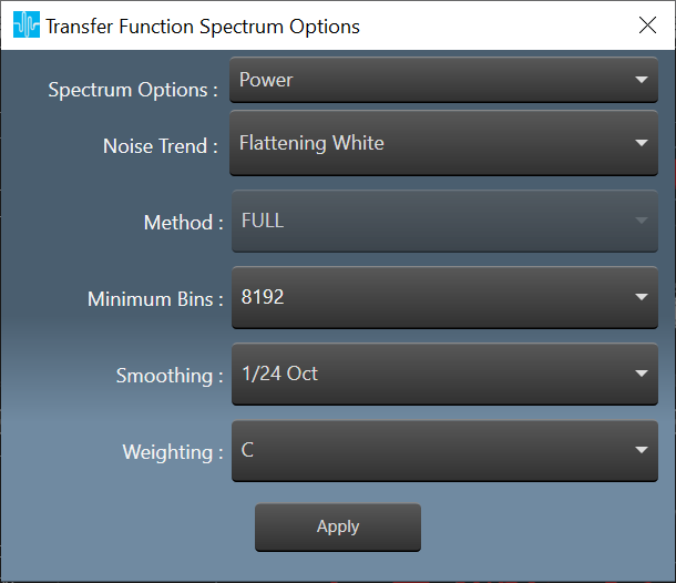
    • A Constant Q transform based on librosa 
      
• Both can change the slope of pink noise (detrend)
  

• WHITE FLAT (default, the power spectrum shows white noise as flat)
  
• PINK FLAT compensates the -3dB/oct behavior of ordinary pink noise (the same noise is detrended in the image). The power of the two spectrums is preserved.
  

• Available Calibrations are:
  

• Digital Values: the compensation constant are not considered, the results and the units are in a.u. (arbitrary unit)
  In MM this is called arbitrary unit a.u. and it is displayed as dBFS
• Calibration  Sound Pressure of the recording in Pa

In Impulse Response Viewer window, you can export acquired measurement to a readable format with the following steps.

Select nodes using checkboxes in left side tree view.

To Select all or un-select all nodes, you can use Select All and Unselect All buttons respectively.

 Inhibit Plotting can be selected to Inhibit plotting graph, it is useful for exporting all or many nodes as on Select All if plotting is on it might take some time to plot graphs

Click Export button as shown in above picture to open Export Data modal dialog,

In the above dialogue window:

• You can provide prefix string and choice of Speaker channel number, which will be part of exported
• Based on your provided options, exported file contains either Impulse response or Transfer Function or both with post processing parameter details and some other details like Audio Configuration, Measured Speakers details, Generator settings etc.
• If you selected “Export as zip” option, all exported content will be zipped under single archived file else dumped out in selected destination folder.
• You can select destination folder (Export Path) using “Browse…” button.
• After providing all your options, click on “Export” button to complete export operation or “Cancel” to close window.
• After export, The destination folder contains separate single file for each selected node with file name in format {AssignedSpeakerChannelNumbers}__{UserPrefix}_{NameOfNode}.meas, in the above case

Different IR Measurements can be averaged  in order to get specific single measurements and those averages can be plotted on graph along with measured sessions and compared.

There are there types of Averaging

• Average with time Alignment
• Average with coherence
• Unweighted average

Right click on In Group to open context menu to Generate Average

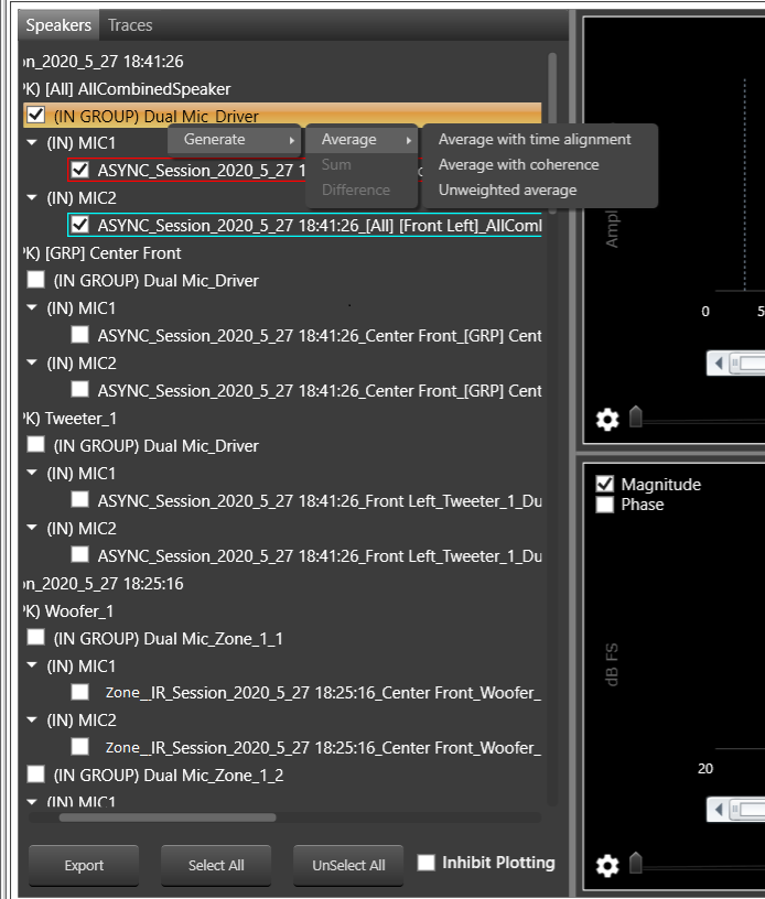
On click of any type of average a window will pop up to enter average curve name

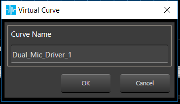
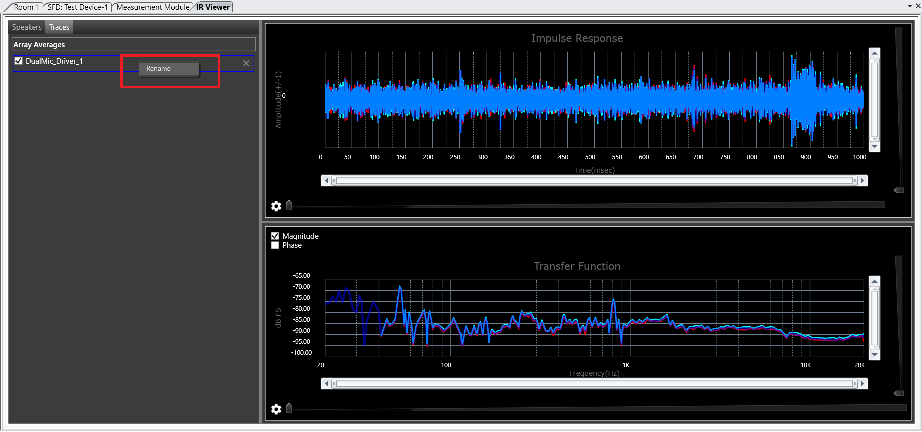
On click of OK , average of selected mics will be created and Time Response and Frequency Response are plotted on graph , Created average curve can be seen in Traces tab under Array Averages.

Already available average curves can be renames using context menu , On Rename a window pop up will open and new name can be assigned there.

User can design target curve using all EQ functions in EQ panel and that can be viewed along with measurements in measurement frequency domain view.

Steps to add Target curve

Click “Add Target Curve” button in Impulse Response viewer.

Configure parameters like sample rate, number of biquads etc in below dialog.

Click “Apply” to continue to design Target Curve in the EQ Panel

Design Target Curve and close panel

Designed curve will be plotted along with measurements in the frequency domain view.

Math operations like Unweighted Average, Sum and Difference can be performed on the Target Curve, as well as derived Target Curves.

Math operation on Target curves :

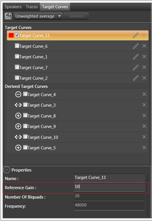
Select math operation from drop down and click “generate” button and resulted curves listed as below

Watch out for icons for summation, average and difference

Reference gain of  Target Curve:

You can update reference gain of Target Curve as shown in below pic and update on Target Curve will plot on graph with updated reference gain.

Selected session can be exported in readable format (json) and/or in .wav file using “Export session” button from measurement in measurement module

On Export Session export settings options window will be opened.

Export settings window includes

• Export Session Name : Session name
• Export as Zip : Option to export session as zip also
• Impulse Response : This can be exported in json and .wav file based on user selection.
• Transfer Function : Option to include/exclude transfer function from export and also transfer functions options selection
• Wav file configuration : Samplerate and Bit depth of wav file can be change by user for wav file export.
• Browse : To browse folder path where exported files will be stored
• Export path : Shows path selected by user

.wav file is manipulated data i.e. selected parameters applied to raw data and saved.

User can alter/modify the Impulse response and Transfer function settings by clicking on the settings icon next to respective check boxes.

On Impulse response settings click Impulse response options will be listed

Window signal options

On click of transfer function settings Transfer functions options will be listed

Transfer function Spectrum options for IR signal type

Transfer function Spectrum options for Recorded signal type

All user selected Impulse response and transfer function settings will be persisted separately for IR and Recorded signal options of  IR/Zone measurements and of Async measurements.

If there is any error during measurement user will be notified with error information

Selected sessions can be exported with raw data into file (button 2) and shared across different projects and can be imported to any project (button 3)

Export Raw Measurement Data

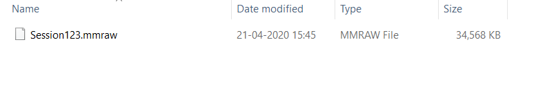
Export raw measurement data button will be enabled when user select one/more sessions and on click of export user will be directed to new modal window where export file name and file path will be requested .On click of Export export file will stored in selected path with .mmraw extension.

This .mmraw file contains exported sessions information and raw data.

To to see exported .wav files

Unzip  exported (Session123.mmraw) file

You can find two files in that  The .SessionInfo file is useful for GTT while importing same raw data. Unzip .mmdata to get .wav files.

Import Raw Measurement Data

.mmdata extensions file is used to import measurements to current project.

If there is session with same session id available inside project already user will be asked to give input to overwrite session or create new session.

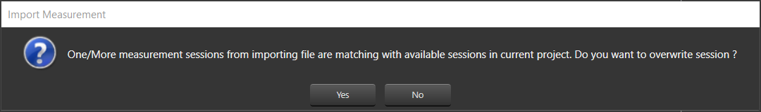
On Yes click old session will be overwritten/replaced by imported sessions .

On No click imported sessions will be created with new session ids.

In any case if imported file session names are already present while importing,  sessions will be imported with new names.

Where user can find Measurement Session Raw data location?

GTT has an option to chose directory to store Measurement Session Raw data as shown in below picture :

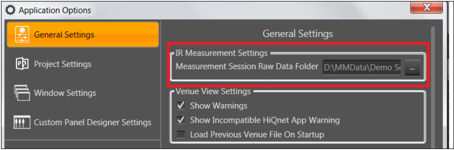
By default directory path is “C:\Users\{CurrentUser}\AppData\Local\Harman\GTT\MeasurementData”  and user can change this path by clicking on “…”(Folder Selection Button).

Problem:

User has created lot of Measurement Sessions and his chosen drive is completely filled now and no more it’s possible to create new Measurement session as there is no room/disk space in chosen drive.

Now user want to move/backup already created Measurement Session data in some other drive.

Solution :

• Move the raw data root folder or content of folder to some other drive .
  For example:a) User has chosen default path to store Measurement Session data , here the root folder will be “MeasurementData”. In this case move the entire “MeasurementData” folder to other drive or move the contents(full or selected folders) of “MeasurementData” folder to other drive (assume “D:\\Measurement _New_Location”)or b) User has chosen the other than default path (C:\\Measurement Session data”) , here root folder is “Measurement Session data”. In this case move the entire “Measurement Session data” folder to other drive or move the contents(full or selected folders) of “Measurement Session data” folder to other drive (assume “D:\\Measurement _New_Location”)
• Now user is succeeded in freeing up space , but GTT is not aware of new raw data location of Session. Hence when user opens Measurement Module the sessions with raw data folder moved to some other location will be marked with “Warning” icon. (Means here the new raw data location needs to be provided).
• To Re-Link session with it’s new raw data location, user has to provide new path(“D:\\Measurement _New_Location”) unsing the Link Measurement Session Data button (number 1).